Learning Note of RL-MDversion

声明

本笔记是在观看赵老师关于强化学习视频做的笔记，原视频移步【一张图讲完强化学习原理】 30分钟了解强化学习的名词脉络_哔哩哔哩_bilibili

作为入门级视频，赵老师将相关数学讲解的十分透彻，强烈建议想要学习RL的初学者将视频刷完，再次感谢赵老师的无私奉献！

概念

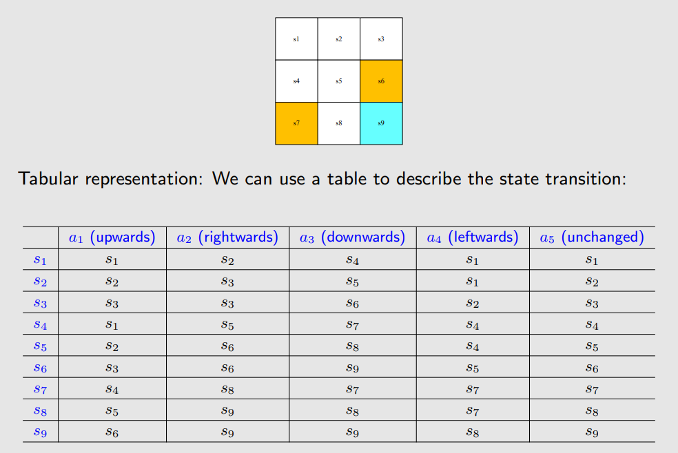
state：状态

state transition：状态改变，可以是确定性的，也可以是不确定性的

$$
\begin{array}{l}
p\left(s_{2} \mid s_{1}, a_{2}\right)=1 \
p\left(s_{i} \mid s_{1}, a_{2}\right)=0 \quad \forall i \neq 2
\end{array}
$$

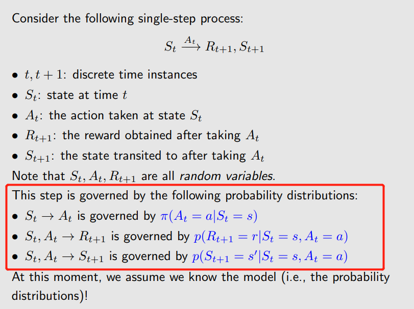
action：某状态采取的动作，可以用条件概率表示

policy：$\pi$:策略

确定性概率：
$$
\begin{array}{l}
\pi\left(a_{1} \mid s_{1}\right)=0 \
\pi\left(a_{2} \mid s_{1}\right)=1 \
\pi\left(a_{3} \mid s_{1}\right)=0 \
\pi\left(a_{4} \mid s_{1}\right)=0 \
\pi\left(a_{5} \mid s_{1}\right)=0
\end{array}
$$
不确定性：同样是概率

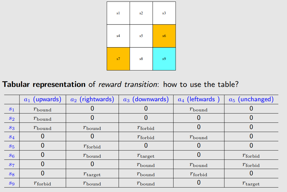
reward：当前状态采取动作对应的奖励/惩罚

return：评价策略好坏，reward总和

discounted return：

1. 防止未来return发散，1+1+1+1+1+1…
2. 平衡现在和未来得到的reward
3. 关于$\gamma$：折扣率，∈[0,1)
4. 接近1，远视；接近0，近视

episode：有限步的一次trial，存在terminal state

continuing tasks：没有terminal state，一直交互

统一方法：将episode转化为continuing，

• 无论什么action都会回到当前状态，或者只有留在原地的action，reward=0
• 设置成普通的状态，reward>0/ <0后续可能会跳出来，更一般

MDP

马尔可夫决策过程

马尔可夫性质：和历史无关，状态转移概率和奖励概率都和历史无关

贝尔曼公式

state value

贝尔曼公式

examples

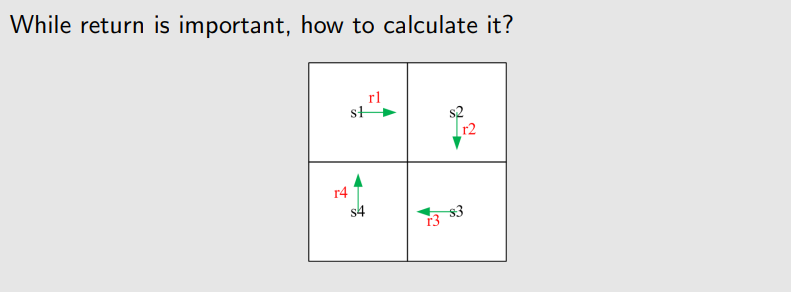
$$
\begin{array}{l}
v_{1}=r_{1}+\gamma\left(r_{2}+\gamma r_{3}+\ldots\right)=r_{1}+\gamma v_{2} \
v_{2}=r_{2}+\gamma\left(r_{3}+\gamma r_{4}+\ldots\right)=r_{2}+\gamma v_{3} \
v_{3}=r_{3}+\gamma\left(r_{4}+\gamma r_{1}+\ldots\right)=r_{3}+\gamma v_{4} \
v_{4}=r_{4}+\gamma\left(r_{1}+\gamma r_{2}+\ldots\right)=r_{4}+\gamma v_{1}
\end{array}
$$
$v_i$表示从某个状态开始计算的return

The returns rely on each other. Bootstrapping!
$$
\underbrace{\left[\begin{array}{l}
v_{1} \
v_{2} \
v_{3} \
v_{4}
\end{array}\right]}{\mathbf{v}}=\left[\begin{array}{l}
r{1} \
r_{2} \
r_{3} \
r_{4}
\end{array}\right]+\left[\begin{array}{l}
\gamma v_{2} \
\gamma v_{3} \
\gamma v_{4} \
\gamma v_{1}
\end{array}\right]=\underbrace{\left[\begin{array}{l}
r_{1} \
r_{2} \
r_{3} \
r_{4}
\end{array}\right]}{\mathbf{r}}+\gamma \underbrace{\left[\begin{array}{llll}
0 & 1 & 0 & 0 \
0 & 0 & 1 & 0 \
0 & 0 & 0 & 1 \
1 & 0 & 0 & 0
\end{array}\right]}{\mathbf{P}} \underbrace{\left[\begin{array}{l}
v_{1} \
v_{2} \
v_{3} \
v_{4}
\end{array}\right]}_{\mathbf{v}}
$$

$$
\mathbf{v}=\mathbf{r}+\gamma \mathbf{P} \mathbf{v}
$$

This is the Bellman equation (for this specific deterministic problem)!!

• Though simple, it demonstrates the core idea: the value of one state relies on the values of other states.

• A matrix-vector form is more clear to see how to solve the state values

state value

discounted return is
$$
G_{t}=R_{t+1}+\gamma R_{t+2}+\gamma^{2} R_{t+3}+\ldots
$$
The expectation (or called expected value or mean) of $G_t$ is defined as the state-value function or simply state value:
$$
v_π(s) = E[G_t|S_t = s]
$$
是关于s的函数，衡量当前状态价值高低，越大说明当前状态价值越高

公式推导

$$
\begin{array}{l}
v_{\pi}(s)=\mathbb{E}\left[R_{t+1} \mid S_{t}=s\right]+\gamma \mathbb{E}\left[G_{t+1} \mid S_{t}=s\right], \ \
=\underbrace{\sum_{a} \pi(a \mid s) \sum_{r} p(r \mid s, a) r}{\text {mean of immediate rewards }}+\underbrace{\gamma \sum{a} \pi(a \mid s) \sum_{s^{\prime}} p\left(s^{\prime} \mid s, a\right) v_{\pi}\left(s^{\prime}\right)}{\text {mean of future rewards }}, \ \
=\sum{a} \pi(a \mid s)\left[\sum_{r} p(r \mid s, a) r+\gamma \sum_{s^{\prime}} p\left(s^{\prime} \mid s, a\right) v_{\pi}\left(s^{\prime}\right)\right], \quad \forall s \in \mathcal{S} \
\end{array}
$$

Matrix vector

Sovle the state values

Given a policy, finding out the corresponding state values is called policy evaluation!

It is a fundamental problem in RL. It is the foundation to find better policies

• closed-form solution
• iterative solution

不同的策略可以得到相同的state value

通过state value可以评价策略好坏

Action value

选择action value大的值的action更新

state value呢？

计算action value：

• 先求state value，再根据公式计算action value
• 直接计算action value

贝尔曼最优公式

贝尔曼公式的特殊情况

• Core concepts: optimal state value and optimal policy

• A fundamental tool: the Bellman optimality equation (BOE)

EXAMPLE

更新：选择action value最大的action

最优策略：每次都选择action value最大的action

原因：贝尔曼最优公式

What if we select the greatest action value? Then, a new policy is obtained:

$$
\pi_{\text {new }}\left(a \mid s_{1}\right)=\left{\begin{array}{ll}
1 & a=a^{} \
0 & a \neq a^{}
\end{array}\right.
$$
where $a^{*}=\arg \max {a} q{\pi}\left(s_{1}, a\right)=a_{3}$ .

Definition

最优策略：A policy $\pi^{}$ is optimal if $v_{\pi^{}}(s) \geq v_{\pi}(s)$ for all s and for any other policy $\pi$ .

The definition leads to many questions:

• Does the optimal policy exist? （所有状态state value都大于其他策略，可能过于理想而不存在）

• Is the optimal policy unique? （是否存在多个最优策略）

• Is the optimal policy stochastic or deterministic? （该策略是确定性还是非确定性）

• How to obtain the optimal policy?（怎么得到）

  To answer these questions, we study the Bellman optimality equation.

BOE

$$
\begin{aligned}
v(s) & =\max {\pi} \sum{a} \pi(a \mid s)\left(\sum_{r} p(r \mid s, a) r+\gamma \sum_{s^{\prime}} p\left(s^{\prime} \mid s, a\right) v\left(s^{\prime}\right)\right), \quad \forall s \in \mathcal{S} \
& =\max _{\pi} \sum \pi(a \mid s) q(s, a) \quad s \in \mathcal{S}
\end{aligned}
$$

若要max，实际是对应最大的 $q(s,a)$

Inspired by the above example, considering that $\sum_{a} \pi(a \mid s)=1$ , we have
$$
\max {\pi} \sum{a} \pi(a \mid s) q(s, a)=\max _{a \in \mathcal{A}(s)} q(s, a)
$$
where the optimality is achieved when

$$
\pi(a \mid s)=\left{\begin{array}{cc}
1 & a=a^{} \
0 & a \neq a^{}
\end{array}\right.
$$
where $a^{*}=\arg \max _{a} q(s, a)$ .

与example处的结果一致

Solve the optimality equation

固定v，求解 $\pi$

实际问题：$v=f(v)$

how to solve the equation?

Contraction mapping theorem

Fixed point（不动点）: $x ∈ X$ is a fixed point of f : $X → X$ if
$$
f(x) = x
$$
Contraction mapping (or contractive function): f is a contraction mapping if
$$
\left|f\left(x_{1}\right)-f\left(x_{2}\right)\right| \leq \gamma\left|x_{1}-x_{2}\right|
$$
where $\gamma \in(0,1) .$

contraction function在求解$x = f(x)$有三点性质

• Existence: there exists a fixed point $x^{} satisfying f\left(x^{}\right)=x^{*} .$
• Uniqueness: The fixed point $x^{*}$ is unique.
• Algorithm: Consider a sequence $\left{x_{k}\right} \space where \space x_{k+1}=f\left(x_{k}\right) , then \space \space x_{k} \rightarrow x^{*}$ as $k \rightarrow \infty$ . Moreover, the convergence rate is exponentially fast.（利用迭代计算出$x_k$, when k-> $\infty$）

solve

对于贝尔曼最优问题，其方程为 contractive function

（证明：满足 $\left|f\left(x_{1}\right)-f\left(x_{2}\right)\right| \leq \gamma\left|x_{1}-x_{2}\right|$ 即可，此处省略证明）

绕路：得到目标奖励越晚！和r等于多少有关，但同时也受到 $\gamma$的约束

因此求解：
$$
\begin{aligned}
v_{k+1}(s) & =\max {\pi} \sum{a} \pi(a \mid s)\left(\sum_{r} p(r \mid s, a) r+\gamma \sum_{s^{\prime}} p\left(s^{\prime} \mid s, a\right) v_{k}\left(s^{\prime}\right)\right) \
& =\max {\pi} \sum{a} \pi(a \mid s) q_{k}(s, a) \
& =\max {a} q{k}(s, a)
\end{aligned}
$$
设立初始的$v_k$，不断迭代得到$v_{k+1}$即可

Example

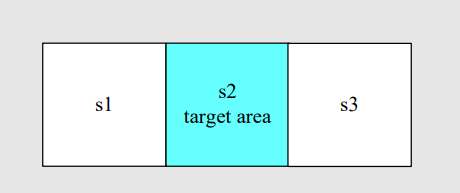
The values of $q(s, a)$
$$
\begin{array}{|c|c|c|c|}
\hline \text { q-value table } & a_{\ell} & a_{0} & a_{r} \
\hline s_{1} & -1+\gamma v\left(s_{1}\right) & 0+\gamma v\left(s_{1}\right) & 1+\gamma v\left(s_{2}\right) \
\hline s_{2} & 0+\gamma v\left(s_{1}\right) & 1+\gamma v\left(s_{2}\right) & 0+\gamma v\left(s_{3}\right) \
\hline s_{3} & 1+\gamma v\left(s_{2}\right) & 0+\gamma v\left(s_{3}\right) & -1+\gamma v\left(s_{3}\right) \
\hline
\end{array}
$$
Consider $\gamma$=0.9 以及下面的初始条件

Our objective is to find $v^{}\left(s_{i}\right)$ and $ \pi^{} k=0$ :
v-value: select $v_{0}\left(s_{1}\right)=v_{0}\left(s_{2}\right)=v_{0}\left(s_{3}\right)=0$

q-value (using the previous table):
$$
\begin{array}{|c|c|c|c|}
\hline & a_{\ell} & a_{0} & a_{r} \
\hline s_{1} & -1 & 0 & 1 \
\hline s_{2} & 0 & 1 & 0 \
\hline s_{3} & 1 & 0 & -1 \
\hline
\end{array}
$$
关于policy：采取greedy policy，select the greatest q-value
$$
\pi\left(a_{r} \mid s_{1}\right)=1, \quad \pi\left(a_{0} \mid s_{2}\right)=1, \quad \pi\left(a_{\ell} \mid s_{3}\right)=1
$$
v-value: $v_{1}(s)=\max {a} q{0}(s, a)$

$$
v_{1}\left(s_{1}\right)=v_{1}\left(s_{2}\right)=v_{1}\left(s_{3}\right)=1
$$
This this policy good? Yes!

但是注意，此时虽然policy是最好的，但是state value没有到最优！！！因为此时k=1，而对应的state value 要到无穷，实际不用到无穷，只需 $|v_{k+1}-v_k|< \sigma$，因此接下来的iteration，k=1
$$
\begin{array}{|c|c|c|c|}
\hline & a_{\ell} & a_{0} & a_{r} \
\hline s_{1} & -0.1 & 0.9 & 1.9 \
\hline s_{2} & 0.9 & 1.9 & 0.9 \
\hline s_{3} & 1.9 & 0.9 & -0.1 \
\hline
\end{array}
$$
然后Greedy policy (select the greatest q-value):
$$
\pi\left(a_{r} \mid s_{1}\right)=1, \quad \pi\left(a_{0} \mid s_{2}\right)=1, \quad \pi\left(a_{\ell} \mid s_{3}\right)=1
$$
k = 2, 3, . . .

Policy optimality

回答上述的问题

Suppose that $v^{*} $ is the unique solution to $v=\max {\pi}\left(r{\pi}+\gamma P_{\pi} v\right) , and v_{\pi}$ is the state value function satisfying $v_{\pi}=r_{\pi}+\gamma P_{\pi} v_{\pi}$ for any given policy $\pi$ , then

$$
v^{} \geq v_{\pi}, \quad \forall \pi
$$
即最优的policy，*对应的state value大于每个地方的state value

同时，最优的policy怎么求？贪心规则

For any $s \in \mathcal{S}$ , the deterministic greedy policy

$$
\pi^{}(a \mid s)=\left{\begin{array}{cc}
1 & a=a^{}(s) \
0 & a \neq a^{*}(s)
\end{array}\right.
$$
is an optimal policy solving the BOE. Here,

$$
a^{}(s)=\arg \max _{a} q^{}(a, s),
$$
where $q^{}(s, a):=\sum_{r} p(r \mid s, a) r+\gamma \sum_{s^{\prime}} p\left(s^{\prime} \mid s, a\right) v^{}\left(s^{\prime}\right) .$

Analyzing optimal policies

即一些有趣的情况

比如 $\gamma$较大时，会比较远视，当$\gamma$较小时，policy 会比较近视

且当reward线性变化时，对应的最优policy不会变化

Value Iteration& Policy Iteration

model-based

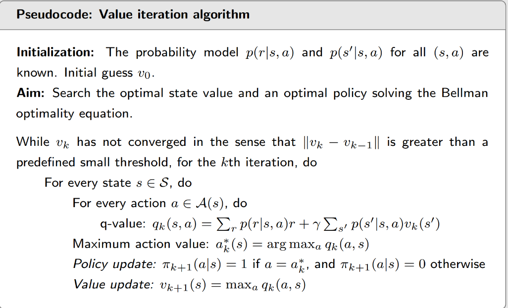
Value iteration

原理

即贝尔曼最优公式的迭代求解法

start from $v_0$

step1：Policy update（PU）

已知 $v_k$，求出q-table，然后找到最大的策略 $\pi_{k+1}$，然后更新
$$
\pi_{k+1}=\arg \max {\pi}\left(r{\pi}+\gamma P_{\pi} v_{k}\right)
$$
step2：value update（VU）

将上面的 $\pi_{k+1}$代入求解 $v_{k+1}$
$$
v_{k+1}=r_{\pi_{k+1}}+\gamma P_{\pi_{k+1}} v_{k}
$$
$v_k$ is not a state value，just a value

实践算法

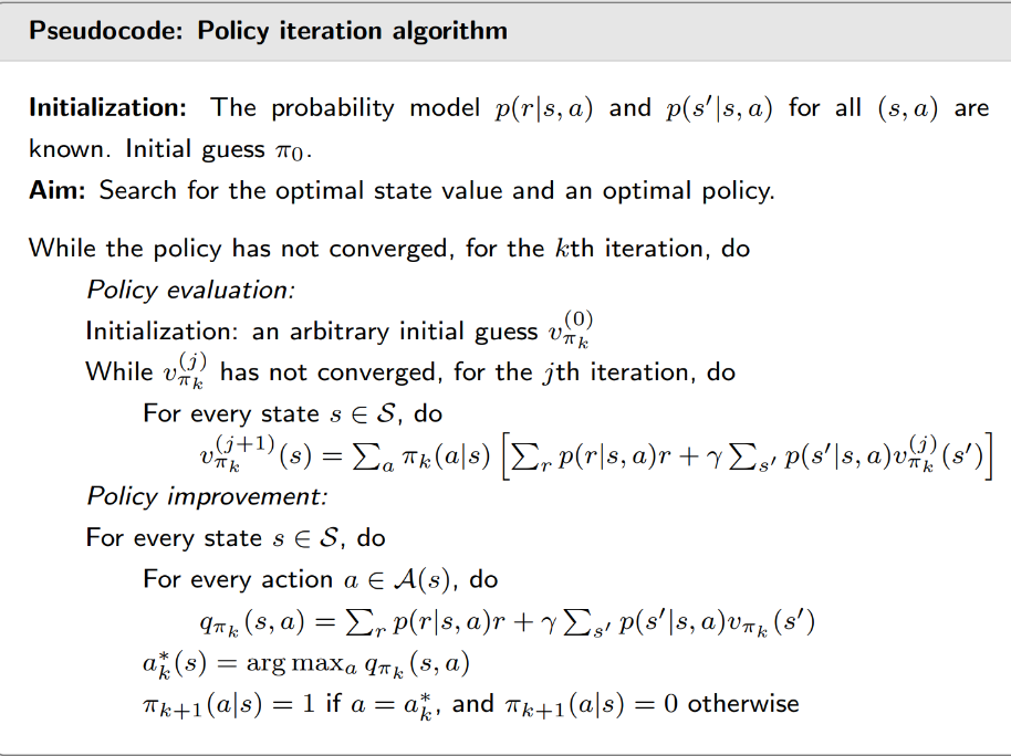
Policy iteration

原理

start from $\pi_0$

step1：policy evaluation（PE）

计算state value，因为state value实际上表征的就是策略的好坏

已知 $\pi_{k}$，求 $v_{\pi k}$

NOTE：此处有两种计算方法，一种是直接计算，一种是迭代计算
$$
v_{\pi_{k}}=r_{\pi_{k}}+\gamma P_{\pi_{k}} v_{\pi_{k}}
$$
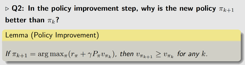
step2：policy improvement（PI）

update policy，用greedy算法得到 $\pi_{k+1}$
$$
\pi_{k+1}=\arg \max {\pi}\left(r{\pi}+\gamma P_{\pi} v_{\pi_{k}}\right)
$$
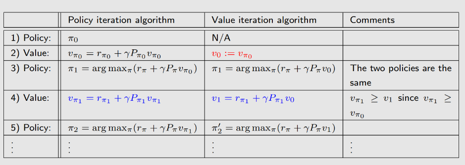
policy iteration 和value iteration的关系

• 证明policy iteration算法收敛时，用到value iteration收敛的结果
• 是 iteration的极端
• 

实践编程算法

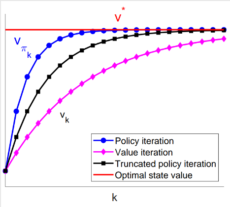
靠近目标的策略会先变好，远离目标的策略会后变好

原因：greedy action，当靠近目标时，target是最greedy的，而greedy则依靠周围的情况，如果周围乱七八糟，得到的策略也不一定是最好的

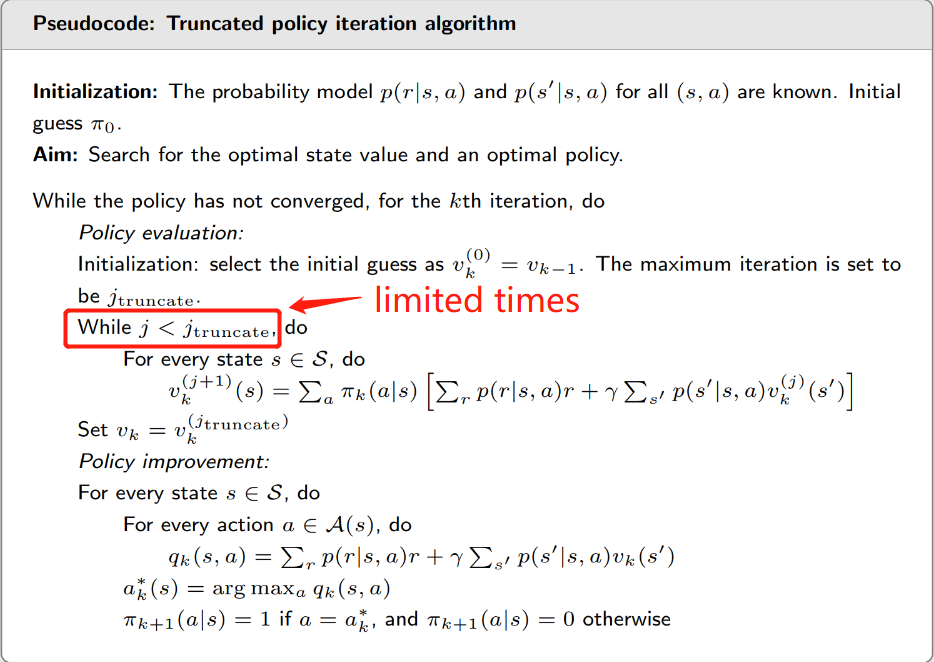
Truncated policy iteration

上述两个算法的一般化！

Consider the step of solving $v_{\pi_{1}}=r_{\pi_{1}}+\gamma P_{\pi_{1}} v_{\pi_{1}}$ :

$$
\begin{aligned}
v_{\pi_{1}}^{(0)} & =v_{0} \
\text { value iteration } \leftarrow v_{1} \longleftarrow v_{\pi_{1}}^{(1)} & =r_{\pi_{1}}+\gamma P_{\pi_{1}} v_{\pi_{1}}^{(0)} \
v_{\pi_{1}}^{(2)} & =r_{\pi_{1}}+\gamma P_{\pi_{1}} v_{\pi_{1}}^{(1)} \
\vdots & \
\text { truncated policy iteration } \leftarrow \bar{v}{1} \longleftarrow v{\pi_{1}}^{(j)} & =r_{\pi_{1}}+\gamma P_{\pi_{1}} v_{\pi_{1}}^{(j-1)} \
\vdots & \
\text { policy iteration } \leftarrow v_{\pi_{1}} \longleftarrow v_{\pi_{1}}^{(\infty)} & =r_{\pi_{1}}+\gamma P_{\pi_{1}} v_{\pi_{1}}^{(\infty)}
\end{aligned}
$$

• The value iteration algorithm computes once.
• The policy iteration algorithm computes an infinite number of iterations.
• The truncated policy iteration algorithm computes a finite number of iterations (say $j$ ). The rest iterations from $j$ to $\infty$ are truncated.

Monte Carlo Learning

Model Free->monte carlo estimation

Core：policy iteration -> model-free

Example

许多次采样！通过平均值来代替期望！数据理论支持：大数定理！

大量实验来近似！为什么蒙特卡罗？因为没有模型，只能实验

Summary：

• Monte Carlo estimation refers to a broad class of techniques that rely
  on repeated random sampling to solve approximation problems.
• Why we care about Monte Carlo estimation? Because it does not
  require the model！
• Why we care about mean estimation? Because state value and action
  value are defined as expectations of random variables！

MC Basic

model-free最大区别的点在于PI中的计算action value

Two expressions of action value:

• Expression 1 requires the model:

$$
q_{\pi_{k}}(s, a)=\sum_{r} p(r \mid s, a) r+\gamma \sum_{s^{\prime}} p\left(s^{\prime} \mid s, a\right) v_{\pi_{k}}\left(s^{\prime}\right)
$$

• Expression 2 does not require the model:

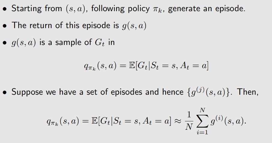
$$
q_{\pi_{k}}(s, a)=\mathbb{E}\left[G_{t} \mid S_{t}=s, A_{t}=a\right]
$$

Idea to achieve model-free RL: We can use expression 2 to calculate $q_{\pi_{k}}(s, a)$ based on data (samples or experiences)!

计算action value

具体Policy iteration

step1: policy evaluation

在求解state value时，用期望代替原本用模型求解的答案

This step is to obtain $q_{\pi_{k}}(s, a)$ for all $(s, a)$ . Specifically, for each action-state pair $(s, a)$ , run an infinite number of (or sufficiently many) episodes. The average of their returns is used to approximate $q_{\pi_{k}}(s, a)$ .

step2：policy improvement

NOTE:

• useful to reveal the core idea，not practical due to low efficiency

• 直接估计action value！而不是估计state value

still is convergent

注意：此处的action value是估计的！

Example1

episode lenth！

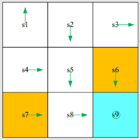
Task:

• An initial policy is shown in the figure.
• Use MC Basic to find the optimal policy.
• $r_{\text {boundary }}=-1, r_{\text {forbidden }}=-1, r_{\text {target }}=1, \gamma=0.9 .$

与model-based区别在哪？不能直接用公式

Step1：policy evaluation

• Since the current policy is deterministic, one episode would be sufficient to get the action value!

• If the current policy is stochastic, an infinite number of episodes (or at least many) are required!（统计计算期望！）

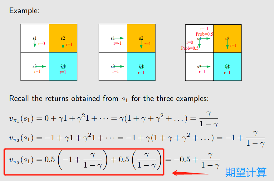
• Starting from $\left(s_{1}, a_{1}\right)$ , the episode is s${1} \stackrel{a{1}}{\longrightarrow} s_{1} \stackrel{a_{1}}{\longrightarrow} s_{1} \stackrel{a_{1}}{\longrightarrow} \ldots$ . Hence, the action value is

$$
q_{\pi_{0}}\left(s_{1}, a_{1}\right)=-1+\gamma(-1)+\gamma^{2}(-1)+\ldots
$$

• Starting from $\left(s_{1}, a_{2}\right)$ , the episode is $s_{1} \stackrel{a_{2}}{\longrightarrow} s_{2} \stackrel{a_{3}}{\longrightarrow} s_{5} \stackrel{a_{3}}{\longrightarrow} \ldots$ . Hence, the action value is

$$
q_{\pi_{0}}\left(s_{1}, a_{2}\right)=0+\gamma 0+\gamma^{2} 0+\gamma^{3}(1)+\gamma^{4}(1)+\ldots
$$

• Starting from $\left(s_{1}, a_{3}\right)$ , the episode is $s_{1} \stackrel{a_{3}}{\longrightarrow} s_{4} \stackrel{a_{2}}{\longrightarrow} s_{5} \stackrel{a_{3}}{\longrightarrow} \ldots$ . Hence, the action value is

$$
q_{\pi_{0}}\left(s_{1}, a_{3}\right)=0+\gamma 0+\gamma^{2} 0+\gamma^{3}(1)+\gamma^{4}(1)+\ldots
$$

Step2：policy improvement

• By observing the action values, we see that

$$
q_{\pi_{0}}\left(s_{1}, a_{2}\right)=q_{\pi_{0}}\left(s_{1}, a_{3}\right)
$$

are the maximum.

• As a result, the policy can be improved as

$$
\pi_{1}\left(a_{2} \mid s_{1}\right)=1 \text { or } \pi_{1}\left(a_{3} \mid s_{1}\right)=1 .
$$

In either way, the new policy for $s_{1}$ becomes optimal.
One iteration is sufficient for this simple example!

Example2

the impact of episode length

所谓episode length，可以理解为探索长度

length=1 -> $q_{\pi_{0}}\left(s_{1}, a_{1}\right)=-1$

length=2 -> $q_{\pi_{0}}\left(s_{1}, a_{1}\right)=-1+\gamma(-1)$

且是从target处开始逆向优化！！

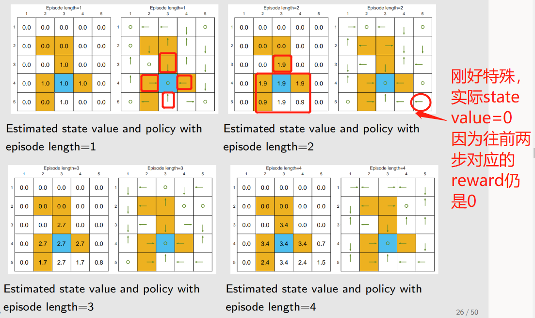
注意上面非0的state value，对应为最优的策略

Conclusion：

• The episode length should be sufficiently long.

• The episode length does not have to be infinitely long.

MC Exploring Start

MC Basic的推广

如何更新？引入Visit！

MC Basic：Initial visit

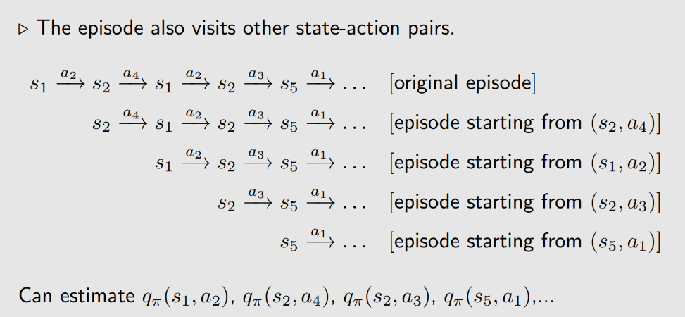
Exploring：在计算一次episode时，其同时访问了其他的state-action pairs，因此可以计算其他的action value，提高效率

Data-efficient methods：

• first-visit method：只用第一次出现的进行估计！
• every-visit method：后面出现的都可以利用来估计！

When to update the policy

• first method：把所有episode的return收集后再开始估计，然后改进

• second method：得到一个episode的return就开始估计，直接改进，得到一个改进一个（最后仍会收敛）

GPI

GPI：generalized policy iteration

• It refers to the general idea or framework of switching between
  policy-evaluation and policy-improvement processes.

• Many model-based and model-free RL algorithms fall into this
  framework.

• 不需要十分精确估计！但最后仍能收敛

Exploring的缺点：每一个state action pair都要有一个episode，以防漏掉

如何解决？看下面！

MC $\xi$-Greedy

为什么要探索？不是按照贪心就可以得到最优策略吗？

为什么用这个策略？不需要exploring starts

Soft policy：A policy is called soft if the probability to take any action is positive.

此处的soft policy：$\xi$-Greedy

原因：episode够长，只要用1个或几个就可以覆盖其他所有state action pair

Definition

$$
\pi(a \mid s)=\left{\begin{array}{ll}1-\frac{\varepsilon}{|\mathcal{A}(s)|}(|\mathcal{A}(s)|-1), & \text { for the greedy action, } \ \frac{\varepsilon}{|\mathcal{A}(s)|}, & \text { for the other }|\mathcal{A}(s)|-1 \text { actions. }\end{array}\right.
$$

where $\varepsilon \in[0,1]$ and $ |\mathcal{A}(s)|$ is the number of actions for s .

• The chance to choose the greedy action is always greater than other actions, because
  $$
  1-\frac{\varepsilon}{|\mathcal{A}(s)|}(|\mathcal{A}(s)|-1)=1-\varepsilon+\frac{\varepsilon}{|\mathcal{A}(s)|} \geq \frac{\varepsilon}{|\mathcal{A}(s)|}
  $$
  .

• Why use $\varepsilon -greedy$? Balance between exploitation and exploration！！！（充分利用和探索性）

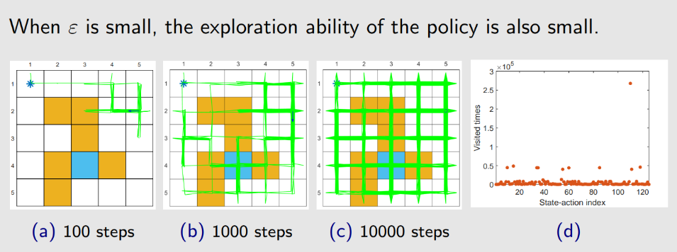
• When $\varepsilon$=0 , it becomes greedy! Less exploration but more exploitation!

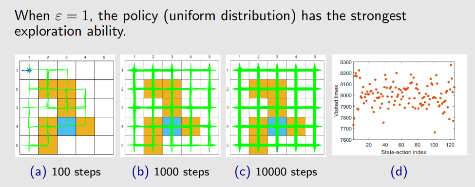
• When $\varepsilon$=1 , it becomes a uniform distribution（均匀分布）. More exploration but less exploitation.

在选择数据时，我们利用every visit，因为action pair可能会被访问很多次，如果用first visit，则会导致数据浪费

Example

Conclusion

• The advantage of $\varepsilon$ -greedy policies is that they have stronger exploration ability so that the exploring starts condition is not required.
• The disadvantage is that $\varepsilon -greedy$ polices are not optimal in general (we can only show that there always exist greedy policies that are optimal).
• The final policy given by the MC $\varepsilon -Greedy$ algorithm is only optimal in the set $\Pi_{\varepsilon}$ of all $\varepsilon -greedy$ policies.
• $\varepsilon$ cannot be too large.
• 当 $\varepsilon$ 为0.1或很小时，得到的policy与greedy policy一致，当变大时，得到的最终的policy与greedy有出入

Stochastic Approximation

Mean estimation Example

how to calculate the mean

• The first way, which is trivial, is to collect all the samples then calculate the average.

• The second way can avoid this drawback because it calculates the average in an incremental and iterative manner.

We can use

$$
w_{k+1}=w_{k}-\frac{1}{k}\left(w_{k}-x_{k}\right) .
$$
to calculate the mean $\bar{x}$ incrementally:(上述公式可推导)

$$
\begin{aligned}
w_{1} & =x_{1} \
w_{2} & =w_{1}-\frac{1}{1}\left(w_{1}-x_{1}\right)=x_{1} \
w_{3} & =w_{2}-\frac{1}{2}\left(w_{2}-x_{2}\right)=x_{1}-\frac{1}{2}\left(x_{1}-x_{2}\right)=\frac{1}{2}\left(x_{1}+x_{2}\right) \
w_{4} & =w_{3}-\frac{1}{3}\left(w_{3}-x_{3}\right)=\frac{1}{3}\left(x_{1}+x_{2}+x_{3}\right) \
& \vdots \
w_{k+1} & =\frac{1}{k} \sum_{i=1}^{k} x_{i}
\end{aligned}
$$
将 $\frac{1}{k}$替换成 $\alpha_k$，即为对应的a special SA algorithm and also a special stochastic gradient descent algorithm

Robbins-Monro algorithm

Description

Stochastic approximation (SA):

• SA is powerful in the sense that it does not require to know the expression of the objective function nor its derivative.

Robbins-Monro (RM) algorithm:

• The is a pioneering work in the field of stochastic approximation.
• The famous stochastic gradient descent algorithm is a special form of the RM algorithm. （SGD）
• It can be used to analyze the mean estimation algorithms introduced in the beginning.

用于求解 $g(w)=0$的解

The Robbins-Monro (RM) algorithm can solve this problem:

$$
w_{k+1}=w_{k}-a_{k} \tilde{g}\left(w_{k}, \eta_{k}\right), \quad k=1,2,3, \ldots
$$
where

• $w_{k}$ is the k th estimate of the root
• $\tilde{g}\left(w_{k}, \eta_{k}\right)=g\left(w_{k}\right)+\eta_{k}$ is the $k th$ noisy observation
• $a_{k}$ is a positive coefficient.($a_k$>0)
  The function $g(w)$ is a black box! This algorithm relies on data:
• Input sequence: $\left{w_{k}\right}$
• Noisy output sequence: $\left{\tilde{g}\left(w_{k}, \eta_{k}\right)\right}$
  Philosophy: without model, we need data!
• Here, the model refers to the expression of the function.

Example

Excise: manually solve $g(w)=w-10$ using the RM algorithm.
Set: $w_{1}=20, a_{k} \equiv 0.5, \eta_{k}=0$ (i.e., no observation error)
$$
\begin{array}{l}
w_{1}=20 \Longrightarrow g\left(w_{1}\right)=10 \
w_{2}=w_{1}-a_{1} g\left(w_{1}\right)=20-0.5 * 10=15 \Longrightarrow g\left(w_{2}\right)=5 \
w_{3}=w_{2}-a_{2} g\left(w_{2}\right)=15-0.5 * 5=12.5 \Longrightarrow g\left(w_{3}\right)=2.5 \
\vdots \
w_{k} \rightarrow 10
\end{array}
$$

Convergence analysis

A rigorous convergence result is given below

Theorem (Robbins-Monro Theorem)
In the Robbins-Monro algorithm, if

1. $0<c_{1} \leq \nabla_{w} g(w) \leq c_{2}$ for all w ;
2. $\sum_{k=1}^{\infty} a_{k}=\infty $and $ \sum_{k=1}^{\infty} a_{k}^{2}<\infty ;$
3. $\mathbb{E}\left[\eta_{k} \mid \mathcal{H}{k}\right]=0$ and $\mathbb{E}\left[\eta{k}^{2} \mid \mathcal{H}{k}\right]<\infty$ ;
   where $\mathcal{H}{k}=\left{w_{k}, w_{k-1}, \ldots\right}$ , then $w_{k}$ converges with probability 1 (w.p.1)(概率收敛) to the root $w^{}$ satisfying $g\left(w^{}\right)=0$

• $a_k$要收敛到0，但不要收敛太快，

Application to mean estimation

estimation algorithm
$$
w_{k+1}=w_{k}+\alpha_{k}\left(x_{k}-w_{k}\right) .
$$
We know that

• If $\alpha_{k}=1 / k$ , then $w_{k+1}=1 / k \sum_{i=1}^{k} x_{i}$ .
• If $\alpha_{k}$ is not $1 / k$ , the convergence was not analyzed.

we show that this algorithm is a special case of the RM algorithm. Then, its convergence naturally follows

下面将证明上述方程为RM算法

1. Consider a function:

$$
g(w) \doteq w-\mathbb{E}[X]
$$

Our aim is to solve $g(w)=0$ . If we can do that, then we can obtain $\mathbb{E}[X]$ .

2. The observation we can get is

$$
\tilde{g}(w, x) \doteq w-x
$$

because we can only obtain samples of X . Note that

$$
\begin{aligned}
\tilde{g}(w, \eta)=w-x & =w-x+\mathbb{E}[X]-\mathbb{E}[X] \
& =(w-\mathbb{E}[X])+(\mathbb{E}[X]-x) \doteq g(w)+\eta,
\end{aligned}
$$

3. The RM algorithm for solving $g(x)=0$ is

$$
w_{k+1}=w_{k}-\alpha_{k} \tilde{g}\left(w_{k}, \eta_{k}\right)=w_{k}-\alpha_{k}\left(w_{k}-x_{k}\right),
$$

which is exactly the mean estimation algorithm.
The convergence naturally follows.

SGD

introduction

SGD is a special RM algorithm.

The mean estimation algorithm is a special SGD algorithm

SGD：常用于解决优化问题(实际还是求根问题？)

最小化：梯度下降

最大化：梯度上升

• GD（gradient descent）

$$
w_{k+1}=w_{k}-\alpha_{k} \nabla_{w} \mathbb{E}\left[f\left(w_{k}, X\right)\right]=w_{k}-\alpha_{k} \mathbb{E}\left[\nabla_{w} f\left(w_{k}, X\right)\right]
$$

drawback： the expected value is difficult to obtain.

• BGD：No model，use data to estimate the mean

$$
\begin{array}{l}
\mathbb{E}\left[\nabla_{w} f\left(w_{k}, X\right)\right] \approx \frac{1}{n} \sum_{i=1}^{n} \nabla_{w} f\left(w_{k}, x_{i}\right)\
w_{k+1}=w_{k}-\alpha_{k} \frac{1}{n} \sum_{i=1}^{n} \nabla_{w} f\left(w_{k}, x_{i}\right) .
\end{array}
$$

Drawback: it requires many samples in each iteration for each $w_k.$

• SGD

• $$
  w_{k+1}=w_{k}-\alpha_{k} \nabla_{w} f\left(w_{k}, x_{k}\right)
  $$

  compared to the BGD, let $n=1$

example

We next consider an example:

$$
\min _{w} \quad J(w)=\mathbb{E}[f(w, X)]=\mathbb{E}\left[\frac{1}{2}|w-X|^{2}\right],
$$
where

$$
f(w, X)=|w-X|^{2} / 2 \quad \nabla_{w} f(w, X)=w-X
$$
answer

• The SGD algorithm for solving the above problem is

$$
w_{k+1}=w_{k}-\alpha_{k} \nabla_{w} f\left(w_{k}, x_{k}\right)=w_{k}-\alpha_{k}\left(w_{k}-x_{k}\right)
$$

• Note:
  • It is the same as the mean estimation algorithm we presented before.
  • That mean estimation algorithm is a special SGD algorithm.

convergence

Core：证明SGD是RM算法，就可以证明其是收敛的

We next show that SGD is a special RM algorithm. Then, the convergence naturally follows.
The aim of SGD is to minimize

$$
J(w)=\mathbb{E}[f(w, X)]
$$
This problem can be converted to a root-finding problem:

$$
\nabla_{w} J(w)=\mathbb{E}\left[\nabla_{w} f(w, X)\right]=0
$$
Let

$$
g(w)=\nabla_{w} J(w)=\mathbb{E}\left[\nabla_{w} f(w, X)\right]
$$
Then, the aim of SGD is to find the root of $g(w)=0$ .

用RM算法解决上述问题

What we can measure is

$$
\begin{aligned}
\tilde{g}(w, \eta) & =\nabla_{w} f(w, x) \ \
& =\underbrace{\mathbb{E}\left[\nabla_{w} f(w, X)\right]}{g(w)}+\underbrace{\nabla{w} f(w, x)-\mathbb{E}\left[\nabla_{w} f(w, X)\right]}_{\eta} .
\end{aligned}
$$
Then, the RM algorithm for solving $g(w)=0$ is

$$
w_{k+1}=w_{k}-a_{k} \tilde{g}\left(w_{k}, \eta_{k}\right)=w_{k}-a_{k} \nabla_{w} f\left(w_{k}, x_{k}\right) \text {. }
$$

• It is exactly the SGD algorithm.
• Therefore, SGD is a special RM algorithm.

pattern

由于梯度具有随机性，收敛是否存在随机性呢？即 $w_k$是否会绕一大圈再回到 $w^{*}$

不存在

通过相对误差来证明
$$
\delta_{k} \doteq \frac{\left|\nabla_{w} f\left(w_{k}, x_{k}\right)-\mathbb{E}\left[\nabla_{w} f\left(w_{k}, X\right)\right]\right|}{\left|\mathbb{E}\left[\nabla_{w} f\left(w_{k}, X\right)\right]\right|}
$$
Since $\mathbb{E}\left[\nabla_{w} f\left(w^{*}, X\right)\right]=0$ , we further have

$$
\delta_{k}=\frac{\left|\nabla_{w} f\left(w_{k}, x_{k}\right)-\mathbb{E}\left[\nabla_{w} f\left(w_{k}, X\right)\right]\right|}{\left|\mathbb{E}\left[\nabla_{w} f\left(w_{k}, X\right)\right]-\mathbb{E}\left[\nabla_{w} f\left(w^{}, X\right)\right]\right|}=\frac{\left|\nabla_{w} f\left(w_{k}, x_{k}\right)-\mathbb{E}\left[\nabla_{w} f\left(w_{k}, X\right)\right]\right|}{\left|\mathbb{E}\left[\nabla_{w}^{2} f\left(\tilde{w}{k}, X\right)\left(w{k}-w^{}\right)\right]\right|} .
$$
上式用了中值定理

where the last equality is due to the mean value theorem and $\tilde{w}{k} \in\left[w{k}, w^{*}\right]$

Suppose $f$ is strictly convex such that

$$
\nabla_{w}^{2} f \geq c>0
$$
for all $w, X ,$ where $c$ is a positive bound.
Then, the denominator of $\delta_{k}$ becomes
$$
\begin{aligned}
\left|\mathbb{E}\left[\nabla_{w}^{2} f\left(\tilde{w}{k}, X\right)\left(w{k}-w^{}\right)\right]\right| & =\left|\mathbb{E}\left[\nabla_{w}^{2} f\left(\tilde{w}{k}, X\right)\right]\left(w{k}-w^{}\right)\right| \
& =\left|\mathbb{E}\left[\nabla_{w}^{2} f\left(\tilde{w}{k}, X\right)\right]\right|\left|\left(w{k}-w^{}\right)\right| \geq c\left|w_{k}-w^{}\right|
\end{aligned}
$$
Substituting the above inequality to $\delta_{k}$ gives

$$
\delta_{k} \leq \frac{|\overbrace{\nabla_{w} f\left(w_{k}, x_{k}\right)}^{\text {stochastic gradient }}-\overbrace{\mathbb{E}\left[\nabla_{w} f\left(w_{k}, X\right)\right]}^{\text {true gradient }}|}{\underbrace{c\left|w_{k}-w^{*}\right|}_{\text {distance to the optimal solution }}} .
$$
因此，

• 当 $w_k$与 $w^{}$相距较远时，分母很大，此时从另外一个角度而言，相对误差很小，分子很小，因此随机梯度和真实梯度基本一致，意味着算法的趋势朝着真实值，也就是 $w^{}$前进

• 当 $w_k$与 $w^{}$相距较近时，分母很小，此时从另外一个角度而言，相对误差较大，分子较大，此时则存在随机性，即其不一定能够准确收敛到 $w^$

因此证明了，不会有收敛的随机性！

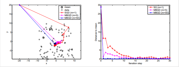
• Although the initial guess of the mean is far away from the true value, the SGD estimate can approach the neighborhood of the true value fast.
• When the estimate is close to the true value, it exhibits certain randomness but still approacwhes the true value gradually

Temporal-Difference Learning

Model-free

迭代式算法

Motivating example

三个例子

First, consider the simple mean estimation problem: calculate
$$
w=\mathbb{E}[X]
$$
based on some iid samples {x} of X .

• By writing $g(w)=w-\mathbb{E}[X]$ , we can reformulate the problem to a root-finding problem

$$
g(w)=0 .
$$

• Since we can only obtain samples {x} of X , the noisy observation is

$$
\tilde{g}(w, \eta)=w-x=(w-\mathbb{E}[X])+(\mathbb{E}[X]-x) \doteq g(w)+\eta .
$$

• Then, according to the last lecture, we know the RM algorithm for solving $g(w)=0$ is

$$
w_{k+1}=w_{k}-\alpha_{k} \tilde{g}\left(w_{k}, \eta_{k}\right)=w_{k}-\alpha_{k}\left(w_{k}-x_{k}\right)
$$

Second
$$
w=\mathbb{E}[v(X)]
$$

$$
\begin{aligned}
g(w) & =w-\mathbb{E}[v(X)] \
\tilde{g}(w, \eta) & =w-v(x)=(w-\mathbb{E}[v(X)])+(\mathbb{E}[v(X)]-v(x)) \doteq g(w)+\eta
\end{aligned}
$$

$$
w_{k+1}=w_{k}-\alpha_{k} \tilde{g}\left(w_{k}, \eta_{k}\right)=w_{k}-\alpha_{k}\left[w_{k}-v\left(x_{k}\right)\right]
$$

Finally
$$
w=\mathbb{E}[R+\gamma v(X)]
$$

$$
w_{k+1}=w_{k}-\alpha_{k} \tilde{g}\left(w_{k}, \eta_{k}\right)=w_{k}-\alpha_{k}\left[w_{k}-\left(r_{k}+\gamma v\left(x_{k}\right)\right)\right]
$$

TD learing of state values

没有模型的情况下，求解贝尔曼公式

求解贝尔曼公式其实就是求解RM算法

Description

The data/experience required by the algorithm:

• $\left(s_{0}, r_{1}, s_{1}, \ldots, s_{t}, r_{t+1}, s_{t+1}, \ldots\right) $ or $ \left{\left(s_{t}, r_{t+1}, s_{t+1}\right)\right}_{t}$ generated following the given policy $\pi$ .

The TD algorithm can be annotated as

$$
\underbrace{v_{t+1}\left(s_{t}\right)}{\text {new estimate }}=\underbrace{v{t}\left(s_{t}\right)}{\text {current estimate }}-\alpha{t}\left(s_{t}\right)[\overbrace{v_{t}\left(s_{t}\right)-[\underbrace{r_{t+1}+\gamma v_{t}\left(s_{t+1}\right)}{\text {TD target } \bar{v}{t}}]}^{\text {TD error } \delta_{t}}],
$$
Here,

$$
\bar{v}{t} \doteq r{t+1}+\gamma v\left(s_{t+1}\right)
$$
is called the TD target.

$$
\delta_{t} \doteq v\left(s_{t}\right)-\left[r_{t+1}+\gamma v\left(s_{t+1}\right)\right]=v\left(s_{t}\right)-\bar{v}{t}
$$
is called the TD error.
It is clear that the new estimate $v{t+1}\left(s_{t}\right)$ is a combination of the current estimate $v_{t}\left(s_{t}\right)$ and the TD error.

TD target 实际就是 $v_{\pi}$，即策略的state value，因为没有模型，最开始并不知道完整的state value，需要不断采样，不断更新，到最后的state value（而不是最优策略）

That is because the algorithm drives $v(s_t)$ towards $\bar v_t$.

TD error

• It is a difference between two consequent time steps.

• It reflects the deficiency between $v_t$ and $v_π$. To see that, denote

$$
\delta_{\pi, t} \doteq v_{\pi}\left(s_{t}\right)-\left[r_{t+1}+\gamma v_{\pi}\left(s_{t+1}\right)\right]
$$

The idea of the algorithm

Q: What does this TD algorithm do mathematically?

A: It solves the Bellman equation of a given policy $π$ without model.

引入新的贝尔曼公式

First, a new expression of the Bellman equation.
The definition of state value of $\pi$ is
$$
v_{\pi}(s)=\mathbb{E}[R+\gamma G \mid S=s], \quad s \in \mathcal{S}
$$
where G is discounted return. Since

$$
\mathbb{E}[G \mid S=s]=\sum_{a} \pi(a \mid s) \sum_{s^{\prime}} p\left(s^{\prime} \mid s, a\right) v_{\pi}\left(s^{\prime}\right)=\mathbb{E}\left[v_{\pi}\left(S^{\prime}\right) \mid S=s\right],
$$
where $S^{\prime}$ is the next state, we can rewrite (4) as

$$
v_{\pi}(s)=\mathbb{E}\left[R+\gamma v_{\pi}\left(S^{\prime}\right) \mid S=s\right], \quad s \in \mathcal{S}
$$
Equation (5) is another expression of the Bellman equation. It is sometimes called the Bellman expectation equation, an important tool to design and analyze TD algorithms.

TD算法是计算贝尔曼公式的一个RM算法

Second, solve the Bellman equation in (5) using the RM algorithm.

In particular, by defining

$$
g(v(s))=v(s)-\mathbb{E}\left[R+\gamma v_{\pi}\left(S^{\prime}\right) \mid s\right],
$$
we can rewrite (5) as

$$
g(v(s))=0
$$
Since we can only obtain the samples $r$ and $s^{\prime}$ of $R$ and $S^{\prime}$ , the noisy observation we have is

$$
\begin{aligned}
\tilde{g}(v(s)) & =v(s)-\left[r+\gamma v_{\pi}\left(s^{\prime}\right)\right] \
& =\underbrace{\left(v(s)-\mathbb{E}\left[R+\gamma v_{\pi}\left(S^{\prime}\right) \mid s\right]\right)}{g(v(s))}+\underbrace{\left(\mathbb{E}\left[R+\gamma v{\pi}\left(S^{\prime}\right) \mid s\right]-\left[r+\gamma v_{\pi}\left(s^{\prime}\right)\right]\right)}{\eta} .
\end{aligned}
$$
therefore
$$
\begin{aligned}
v{k+1}(s) & =v_{k}(s)-\alpha_{k} \tilde{g}\left(v_{k}(s)\right) \
& =v_{k}(s)-\alpha_{k}\left(v_{k}(s)-\left[r_{k}+\gamma v_{\pi}\left(s_{k}^{\prime}\right)\right]\right), \quad k=1,2,3, \ldots
\end{aligned}
$$
To remove the two assumptions in the RM algorithm, we can modify it

• One modification is that $\left{\left(s, r, s^{\prime}\right)\right}$ is changed to $\left{\left(s_{t}, r_{t+1}, s_{t+1}\right)\right}$ so that the algorithm can utilize the sequential samples in an episode.
• Another modification is that $v_{\pi}\left(s^{\prime}\right)$ is replaced by an estimate of it because we don’t know it in advance.

convergence

Theorem (Convergence of TD Learning)
By the TD algorithm (1), $v_{t}(s)$ converges with probability 1 to $v_{\pi}(s)$ for all $s \in \mathcal{S}$ as $t \rightarrow \infty$ if $\sum_{t} \alpha_{t}(s)=\infty$ and $\sum_{t} \alpha_{t}^{2}(s)<\infty$ for all $s \in \mathcal{S}$ .

Comparison

$$
\begin{array}{l|l}
\hline \hline \text { TD/Sarsa learning } & \text { MC learning } \
\hline \begin{array}{l}
\text { Online: TD learning is online. It can } \
\text { update the state/action values imme- } \
\text { diately after receiving a reward. }
\end{array} & \begin{array}{l}
\text { Offline: MC learning is offline. It } \
\text { has to wait until an episode has been } \
\text { completely collected. }
\end{array} \
\hline \begin{array}{l}
\text { Continuing tasks: Since TD learning } \
\text { is online, it can handle both episodic } \
\text { and continuing tasks. }
\end{array} &
\begin{array}{l}
\text { Episodic tasks } \
\text { is offline, it can only handle episodic } \
\text { tasks that has terminate states. }
\end{array} \
\hline
\end{array}
$$

$$
\begin{array}{l|l}
\hline \text { TD/Sarsa learning } & \text { MC learning } \
\hline \begin{array}{l}
\text { Bootstrapping: TD bootstraps be- } \
\text { cause the update of a value relies on } \
\text { the previous estimate of this value. } \
\text { Hence, it requires initial guesses. }
\end{array} & \begin{array}{l}
\text { Non-bootstrapping: MC is not } \
\text { bootstrapping, because it can directly } \
\text { estimate state/action values without } \
\text { any initial guess. }
\end{array} \
\hline \begin{array}{l}
\text { Low estimation variance: TD has } \
\text { lower than MC because there are few- } \
\text { er random variables. For instance, } \
\text { Sarsa requires } R_{t+1}, S_{t+1}, A_{t+1} .
\end{array} & \begin{array}{l}
\text { High estimation variance: To esti- } \
\text { mate } q_{\pi}\left(s_{t}, a_{t}\right), \text { we need samples of } \
R_{t+1}+\gamma R_{t+2}+\gamma^{2} R_{t+3}+\ldots \text { Sup- } \
\text { pose the length of each episode is } L . \
\text { There are }|\mathcal{A}|^{L} \text { possible episodes. }
\end{array} \
\hline
\end{array}
$$

Sarsa

Description

Core Idea：that is to use an algorithm to solve the Bellman equation of a given policy.

The complication emerges when we try to find optimal policies and work efficiently

Next, we introduce, Sarsa, an algorithm that can directly estimate action values.

估计action value，从而更新，改进策略，Policy evaluation+Policy improvement

如何估计呢？not model，need data

也是求解了一个action value相关的贝尔曼公式！

收敛性：$q_t(s,a) -> q_\pi(s,a)$

在policy evaluation（update q-value） 后立马policy improvement（update policy）

First, our aim is to estimate the action values of a given policy $\pi$ .
Suppose we have some experience $\left{\left(s_{t}, a_{t}, r_{t+1}, s_{t+1}, a_{t+1}\right)\right}_{t}$ .（Sarsa）

We can use the following Sarsa algorithm to estimate the action values:
$$
\begin{aligned}
q_{t+1}\left(s_{t}, a_{t}\right) & =q_{t}\left(s_{t}, a_{t}\right)-\alpha_{t}\left(s_{t}, a_{t}\right)\left[q_{t}\left(s_{t}, a_{t}\right)-\left[r_{t+1}+\gamma q_{t}\left(s_{t+1}, a_{t+1}\right)\right]\right], \
q_{t+1}(s, a) & =q_{t}(s, a), \quad \forall(s, a) \neq\left(s_{t}, a_{t}\right),
\end{aligned}
$$
where $t=0,1,2, \ldots$

NOTE：第二个条件是当某个state action pair没被访问时，将保持原状

• $q_{t}\left(s_{t}, a_{t}\right)$ is an estimate of $q_{\pi}\left(s_{t}, a_{t}\right)$ ;
• $\alpha_{t}\left(s_{t}, a_{t}\right)$ is the learning rate depending on $s_{t}, a_{t}$ .

如何policy improvement？

For each episode, do

• If the current $s_{t}$ is not the target state, do
  • Collect the experience $\left(s_{t}, a_{t}, r_{t+1}, s_{t+1}, a_{t+1}\right)$ : In particular, take action $a_{t}$ following $\pi_{t}\left(s_{t}\right)$ , generate $r_{t+1}, s_{t+1}$ , and then take action $a_{t+1}$ following $\pi_{t}\left(s_{t+1}\right) .$
  • Update q-value（policy evaluation）:

$$
\begin{array}{l}
q_{t+1}\left(s_{t}, a_{t}\right)=q_{t}\left(s_{t}, a_{t}\right)-\alpha_{t}\left(s_{t}, a_{t}\right)\left[q_{t}\left(s_{t}, a_{t}\right)-\left[r_{t+1}+\right.\right.
\left.\gamma q_{t}\left(s_{t+1}, a_{t+1}\right)\right]
\end{array}
$$

• • Update policy（policy ）:

$$
\begin{array}{l}
\pi_{t+1}\left(a \mid s_{t}\right)=1-\frac{\epsilon}{|\mathcal{A}|}(|\mathcal{A}|-1) \text { if } a=\arg \max {a} q{t+1}\left(s_{t}, a\right) \
\pi_{t+1}\left(a \mid s_{t}\right)=\frac{\epsilon}{|\mathcal{A}|} \text { otherwise }
\end{array}
$$

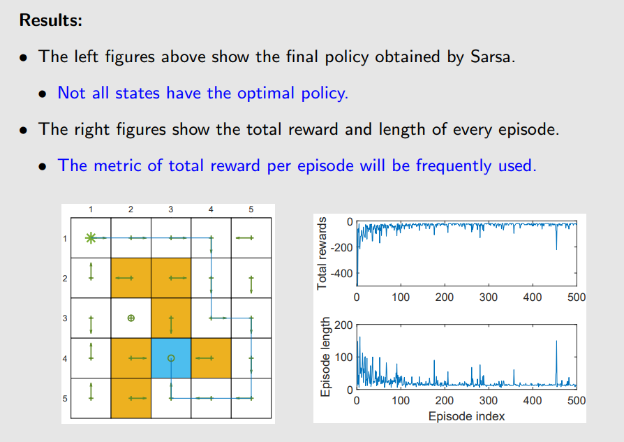
Example

The task is to find a good path from a specific starting state to the target state

So:

Expected Sarsa

Description

A variant of Sarsa is the Expected Sarsa algorithm:

$$
\begin{aligned}
q_{t+1}\left(s_{t}, a_{t}\right) & =q_{t}\left(s_{t}, a_{t}\right)-\alpha_{t}\left(s_{t}, a_{t}\right)\left[q_{t}\left(s_{t}, a_{t}\right)-\left(r_{t+1}+\gamma \mathbb{E}\left[q_{t}\left(s_{t+1}, A\right)\right]\right)\right], \
q_{t+1}(s, a) & =q_{t}(s, a), \quad \forall(s, a) \neq\left(s_{t}, a_{t}\right),
\end{aligned}
$$
where

$$
\left.\mathbb{E}\left[q_{t}\left(s_{t+1}, A\right)\right]\right)=\sum_{a} \pi_{t}\left(a \mid s_{t+1}\right) q_{t}\left(s_{t+1}, a\right) \doteq v_{t}\left(s_{t+1}\right)
$$
is the expected value of $q_{t}\left(s_{t+1}, a\right)$ under policy $\pi_{t}$ .
Compared to Sarsa:

• The TD target is changed from $r_{t+1}+\gamma q_{t}\left(s_{t+1}, a_{t+1}\right)$ as in Sarsa to $r_{t+1}+\gamma \mathbb{E}\left[q_{t}\left(s_{t+1}, A\right)\right]$ as in Expected Sarsa.
• Need more computation. But it is beneficial in the sense that it reduces the estimation variances because it reduces random variables in Sarsa from $\left{s_{t}, a_{t}, r_{t+1}, s_{t+1}, a_{t+1}\right} $ to $\left{s_{t}, a_{t}, r_{t+1}, s_{t+1}\right} .$（因为遍历了所有的action）

n-step Sarsa

n -step Sarsa: can unify Sarsa and Monte Carlo learning The definition of action value is

$$
\begin{array}{l}
\text { Sarsa } \longleftarrow \quad G_{t}^{(1)}=R_{t+1}+\gamma q_{\pi}\left(S_{t+1}, A_{t+1}\right), \
G_{t}^{(2)}=R_{t+1}+\gamma R_{t+2}+\gamma^{2} q_{\pi}\left(S_{t+2}, A_{t+2}\right), \
\vdots \
n \text {-step Sarsa } \longleftarrow \quad G_{t}^{(n)}=R_{t+1}+\gamma R_{t+2}+\cdots+\gamma^{n} q_{\pi}\left(S_{t+n}, A_{t+n}\right), \
\vdots \
\text { MC } \longleftarrow \quad G_{t}^{(\infty)}=R_{t+1}+\gamma R_{t+2}+\gamma^{2} R_{t+3}+\ldots
\end{array}
$$

• Sarsa aims to solve

$$
q_{\pi}(s, a)=\mathbb{E}\left[G_{t}^{(1)} \mid s, a\right]=\mathbb{E}\left[R_{t+1}+\gamma q_{\pi}\left(S_{t+1}, A_{t+1}\right) \mid s, a\right] .
$$

• MC learning aims to solve

$$
q_{\pi}(s, a)=\mathbb{E}\left[G_{t}^{(\infty)} \mid s, a\right]=\mathbb{E}\left[R_{t+1}+\gamma R_{t+2}+\gamma^{2} R_{t+3}+\ldots \mid s, a\right] .
$$

• An intermediate algorithm called n -step Sarsa aims to solve

• $$
  q_{\pi}(s, a)=\mathbb{E}\left[G_{t}^{(n)} \mid s, a\right]=\mathbb{E}\left[R_{t+1}+\gamma R_{t+2}+\cdots+\gamma^{n} q_{\pi}\left(S_{t+n}, A_{t+n}\right) \mid s, a\right]

  • $$

  The algorithm of n -step Sarsa is

$$
\begin{aligned}
q_{t+1}\left(s_{t}, a_{t}\right)= & q_{t}\left(s_{t}, a_{t}\right)
-\alpha_{t}\left(s_{t}, a_{t}\right)\left[q_{t}\left(s_{t}, a_{t}\right)-\left[r_{t+1}+\gamma r_{t+2}+\cdots+\gamma^{n} q_{t}\left(s_{t+n}, a_{t+n}\right)\right]\right] .
\end{aligned}
$$

n -step Sarsa is more general because it becomes the (one-step) Sarsa algorithm when $n=1$ and the MC learning algorithm when $n=\infty .$

Q-learning

Description

Core Idea：求解贝尔曼最优公式
$$
\begin{aligned}
q_{t+1}\left(s_{t}, a_{t}\right) & =q_{t}\left(s_{t}, a_{t}\right)-\alpha_{t}\left(s_{t}, a_{t}\right)\left[q_{t}\left(s_{t}, a_{t}\right)-\left[r_{t+1}+\gamma \max {a \in \mathcal{A}} q{t}\left(s_{t+1}, a\right)\right]\right], \
q_{t+1}(s, a) & =q_{t}(s, a), \quad \forall(s, a) \neq\left(s_{t}, a_{t}\right)
\end{aligned}
$$
引入了 behavior policy，target policy

==offline 怎么更新 pi_b==(看原书)

off-Policy Vs on-policy

off-policy：比如我behavior policy可以用探索性比较强的，比如action的选择可以均匀分布，以此来得到更多experience

而对应的target policy为了得到最优的策略，直接选择greedy policy，而不是 $\varepsilon$-greedy，因为此时我已经不缺探索性了

on-policy：而behavior policy=target policy，比如 Sarsa，uses $\varepsilon$-greedy policies to maintain certain exploration ability, 但由于一般设置较小，其对应的探索能力有限，因为如果设置较大，最后优化效果并不好

Value Function

Example

Core Idea：用曲线拟合替代tables 表示state value

最简单：直线拟合
$$
\hat{v}(s, w)=a s+b=\underbrace{[s, 1]}{\phi^{T}(s)} \underbrace{\left[\begin{array}{l}
a \
b
\end{array}\right]}{w}=\phi^{T}(s) w
$$
where

• $w$ is the parameter vector
• $\phi(s)$ the feature vector of $s$
• $\hat{v}(s, w)$ is linear in $w$

当然，也可以用二阶，三阶，高阶拟合
$$
\hat{v}(s, w)=a s^{2}+b s+c=\underbrace{\left[s^{2}, s, 1\right]}{\phi^{T}(s)} \underbrace{\left[\begin{array}{c}
a \
b \
c
\end{array}\right]}{w}=\phi^{T}(s) w .
$$
优点：存储方面，存储的维数大幅减少，

同时，泛化能力很好

When a state s is visited, the parameter $w$ is updated so that the values of some other unvisited states can also be updated.

Algorithm for state value estimation

Objective function

The objective function is

$$
J(w)=\mathbb{E}\left[\left(v_{\pi}(S)-\hat{v}(S, w)\right)^{2}\right]
$$

• Our goal is to find the best $w$ that can minimize $J(w)$ .
• The expectation is with respect to the random variable $S \in \mathcal{S}$ . What is the probability distribution of $S$ ?
• This is often confusing because we have not discussed the probability distribution of states so far in this book.
• There are several ways to define the probability distribution of $S$ .

first way：uniform distribution
$$
J(w)=\mathbb{E}\left[\left(v_{\pi}(S)-\hat{v}(S, w)\right)^{2}\right]=\frac{1}{|\mathcal{S}|} \sum_{s \in \mathcal{S}}\left(v_{\pi}(s)-\hat{v}(s, w)\right)^{2}
$$
缺点：有些状态离target area较远，并不重要，被访问次数较少，对应的权重应小

second way：stationary distribution.

Let $\left{d_{\pi}(s)\right}{s \in \mathcal{S}}$ denote the stationary distribution of the Markov process under policy $\pi$ . By definition, $d{\pi}(s) \geq 0$ and $\sum_{s \in \mathcal{S}} d_{\pi}(s)=1$ .
$$
J(w)=\mathbb{E}\left[\left(v_{\pi}(S)-\hat{v}(S, w)\right)^{2}\right]=\sum_{s \in \mathcal{S}} d_{\pi}(s)\left(v_{\pi}(s)-\hat{v}(s, w)\right)^{2}
$$
为什么叫稳态？因为要足够多次的step，等系统稳定后，基本不再改变时

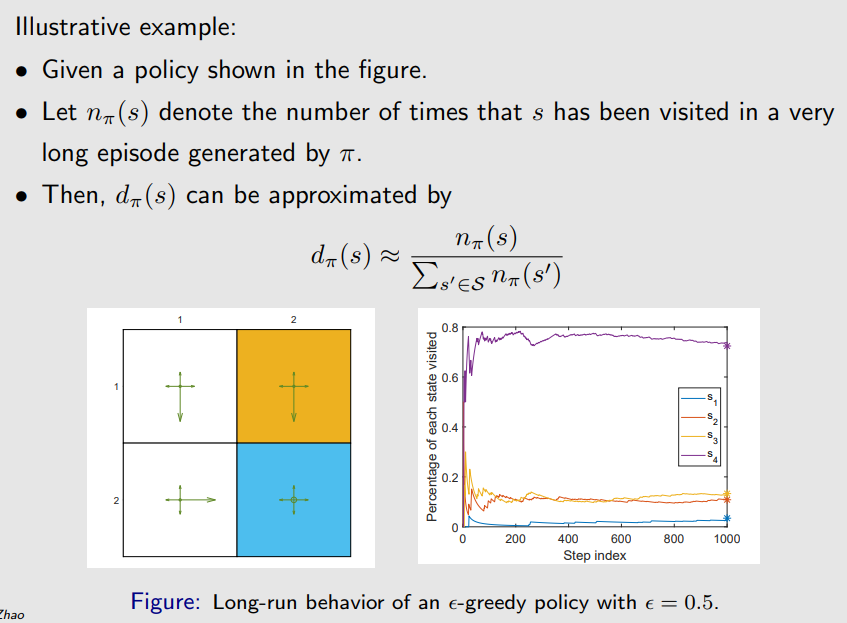
可以证明，最后的 $d_\pi(s)$为转移矩阵的特征向量

[Book All-in-one.pdf](file:///D:/desktop/Bing_DownLoad/Book All-in-one.pdf)

Optimization algorithms

那究竟如何优化呢？

最小化：梯度下降
$$
w_{k+1}=w_{k}-\alpha_{k} \nabla_{w} J\left(w_{k}\right)
$$
The true gradient is

$$
\begin{aligned}
\nabla_{w} J(w) & =\nabla_{w} \mathbb{E}\left[\left(v_{\pi}(S)-\hat{v}(S, w)\right)^{2}\right] \
& =\mathbb{E}\left[\nabla_{w}\left(v_{\pi}(S)-\hat{v}(S, w)\right)^{2}\right] \
& =2 \mathbb{E}\left[\left(v_{\pi}(S)-\hat{v}(S, w)\right)\left(-\nabla_{w} \hat{v}(S, w)\right)\right] \
& =-2 \mathbb{E}\left[\left(v_{\pi}(S)-\hat{v}(S, w)\right) \nabla_{w} \hat{v}(S, w)\right]
\end{aligned}
$$
use the stochastic gradient
$$
w_{t+1}=w_{t}+\alpha_{t}\left(v_{\pi}\left(s_{t}\right)-\hat{v}\left(s_{t}, w_{t}\right)\right) \nabla_{w} \hat{v}\left(s_{t}, w_{t}\right)
$$
系数2已经合并到常数里了

注意到 $v_\pi$未知，因此要进行替代

两种替代方式：Monte Carlo learning和TD Learning（但是此种替代并不严谨，优化的并不是上述true error，而是projected Bellman error）

• First, Monte Carlo learning with function approximation
  Let $g_{t}$ be the discounted return starting from $s_{t}$ in the episode. Then, $g_{t}$ can be used to approximate $v_{\pi}\left(s_{t}\right)$ . The algorithm becomes

$$
w_{t+1}=w_{t}+\alpha_{t}\left(g_{t}-\hat{v}\left(s_{t}, w_{t}\right)\right) \nabla_{w} \hat{v}\left(s_{t}, w_{t}\right)
$$

• Second, TD learning with function approximation
  By the spirit of TD learning, $r_{t+1}+\gamma \hat{v}\left(s_{t+1}, w_{t}\right)$ can be viewed as an approximation of $v_{\pi}\left(s_{t}\right)$ . Then, the algorithm becomes

$$
w_{t+1}=w_{t}+\alpha_{t}\left[r_{t+1}+\gamma \hat{v}\left(s_{t+1}, w_{t}\right)-\hat{v}\left(s_{t}, w_{t}\right)\right] \nabla_{w} \hat{v}\left(s_{t}, w_{t}\right)
$$

Selection of function approximators

究竟如何选择相关函数，1阶？2阶？

一阶的好处：简洁，参数少

• The theoretical properties of the TD algorithm in the linear case can be much better understood than in the nonlinear case.

• Linear function approximation is still powerful in the sense that the tabular representation is merely a special case of linear function approximation.

坏处：难以拟合非线性情况

Recall that the TD-Linear algorithm is

$$
w_{t+1}=w_{t}+\alpha_{t}\left[r_{t+1}+\gamma \phi^{T}\left(s_{t+1}\right) w_{t}-\phi^{T}\left(s_{t}\right) w_{t}\right] \phi\left(s_{t}\right),
$$

• When $\phi\left(s_{t}\right)=e_{s}$ , the above algorithm becomes

$$
w_{t+1}=w_{t}+\alpha_{t}\left(r_{t+1}+\gamma w_{t}\left(s_{t+1}\right)-w_{t}\left(s_{t}\right)\right) e_{s_{t}} .
$$

This is a vector equation that merely updates the $s_{t}$ th entry of $w_{t}$ .

• Multiplying $e_{s_{t}}^{T}$ on both sides of the equation gives

$$
w_{t+1}\left(s_{t}\right)=w_{t}\left(s_{t}\right)+\alpha_{t}\left(r_{t+1}+\gamma w_{t}\left(s_{t+1}\right)-w_{t}\left(s_{t}\right)\right),
$$

which is exactly the tabular TD algorithm.

Examples

Summary of the story

theoretical analysis

• The algorithm

$$
w_{t+1}=w_{t}+\alpha_{t}\left[r_{t+1}+\gamma \hat{v}\left(s_{t+1}, w_{t}\right)-\hat{v}\left(s_{t}, w_{t}\right)\right] \nabla_{w} \hat{v}\left(s_{t}, w_{t}\right)
$$

does not minimize the following objective function:

$$
J(w)=\mathbb{E}\left[\left(v_{\pi}(S)-\hat{v}(S, w)\right)^{2}\right]
$$

Different objective functions:

• Objective function 1: True value error

$$
J_{E}(w)=\mathbb{E}\left[\left(v_{\pi}(S)-\hat{v}(S, w)\right)^{2}\right]=\left|\hat{v}(w)-v_{\pi}\right|_{D}^{2}
$$

• Objective function 2: Bellman error

$$
J_{B E}(w)=\left|\hat{v}(w)-\left(r_{\pi}+\gamma P_{\pi} \hat{v}(w)\right)\right|{D}^{2} \doteq\left|\hat{v}(w)-T{\pi}(\hat{v}(w))\right|_{D}^{2}
$$

where $T_{\pi}(x) \doteq r_{\pi}+\gamma P_{\pi} x$

• Objective function 3: Projected Bellman error

$$
J_{P B E}(w)=\left|\hat{v}(w)-M T_{\pi}(\hat{v}(w))\right|_{D}^{2}
$$

where $M$ is a **projection matrix.**（投影变换矩阵，即无论 $w$怎么选，两者都有距离时，该投影变换矩阵能将二者error变为0）
The TD-Linear algorithm minimizes the projected Bellman error.
Details can be found in the book.

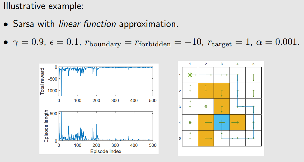
Sarsa with function approximation

Core Idea：利用Sarsa估计action value

So far, we merely considered the problem of state value estimation. That is we hope

$$
\hat{v} \approx v_{\pi}
$$
To search for optimal policies, we need to estimate action values.
The Sarsa algorithm with value function approximation is
$$
w_{t+1}=w_{t}+\alpha_{t}\left[r_{t+1}+\gamma \hat{q}\left(s_{t+1}, a_{t+1}, w_{t}\right)-\hat{q}\left(s_{t}, a_{t}, w_{t}\right)\right] \nabla_{w} \hat{q}\left(s_{t}, a_{t}, w_{t}\right) \text {. }
$$
This is the same as the algorithm we introduced previously in this lecture except that $\hat{v}$ is replaced by $\hat{q} .$

Q-learning with function approximation

Core Idea：利用q-learning的方式更新action value

The q-value update rule is

$$
w_{t+1}=w_{t}+\alpha_{t}\left[r_{t+1}+\gamma \max {a \in \mathcal{A}\left(s{t+1}\right)} \hat{q}\left(s_{t+1}, a, w_{t}\right)-\hat{q}\left(s_{t}, a_{t}, w_{t}\right)\right] \nabla_{w} \hat{q}\left(s_{t}, a_{t}, w_{t}\right)
$$
which is the same as Sarsa except that $\hat{q}\left(s_{t+1}, a_{t+1}, w_{t}\right)$ is replaced by $\max {a \in \mathcal{A}\left(s{t+1}\right)} \hat{q}\left(s_{t+1}, a, w_{t}\right)$

Deep Q-learning

DQN：原本算法计算变量梯度，涉及到神经网络底层，因此要进行改进

Deep Q-learning aims to minimize the objective function/loss function:

$$
J(w)=\mathbb{E}\left[\left(R+\gamma \max _{a \in \mathcal{A}\left(S^{\prime}\right)} \hat{q}\left(S^{\prime}, a, w\right)-\hat{q}(S, A, w)\right)^{2}\right],
$$
where $\left(S, A, R, S^{\prime}\right)$ are random variables.

• This is actually the Bellman optimality error. That is because

$$
q(s, a)=\mathbb{E}\left[R_{t+1}+\gamma \max {a \in \mathcal{A}\left(S{t+1}\right)} q\left(S_{t+1}, a\right) \mid S_{t}=s, A_{t}=a\right], \quad \forall s, a
$$

The value of $R+\gamma \max _{a \in \mathcal{A}\left(S^{\prime}\right)} \hat{q}\left(S^{\prime}, a, w\right)-\hat{q}(S, A, w)$ should be zero in the expectation sense

均匀采样的数学原因：

Policy Function

Core Idea：函数表达策略！

value-based to policy based

优化目标函数来求最优策略

$\theta$是参数，可以是神经网络，用以计算 $\pi(a|s)$

Basic idea of Policy gradient

The basic idea of the policy gradient is simple:

• First, metrics (or objective functions) to define optimal policies: $J(\theta)$ , which can define optimal policies.（定义目标函数）
• Second, gradient-based optimization algorithms to search for optimal policies:（优化目标函数）

$$
\theta_{t+1}=\theta_{t}+\alpha \nabla_{\theta} J\left(\theta_{t}\right)
$$

Although the idea is simple, the complication emerges when we try to answer the following questions.

• What appropriate metrics should be used?（选择什么函数合适）
• How to calculate the gradients of the metrics?（如何优化？）

Metrics to define optimal policies

Two metrics（两种优化函数）

都是关于 $\pi$的函数，且 $\pi$是 $\theta$的函数

The first metric is the average state value or simply called average value

Average value

求出每个state的state value然后求mean
$$
\bar{v}{\pi}=\sum{s \in \mathcal{S}} d(s) v_{\pi}(s)
$$

• $\bar{v}_{\pi}$ is a weighted average of the state values.
• $d(s) \geq 0$ is the weight for state $s$ .
• Since $\sum_{s \in \mathcal{S}} d(s)=1$ , we can interpret $d(s)$ as a probability distribution. Then, the metric can be written as

$$
\bar{v}{\pi}=\mathbb{E}\left[v{\pi}(S)\right]
$$

where $S \sim d .$

How to select the distribution d? There are two cases.

• The first case is that $d$ is independent of the policy $π$.（另外一种就是依赖于决策）

不依赖又分两种：均匀（equally important）和非均匀（ only interested in a specific state $s_0$）

we only care about the long-term return starting from $s_0$
$$
d_{0}\left(s_{0}\right)=1, \quad d_{0}\left(s \neq s_{0}\right)=0
$$

• The second case is that $d$ depends on the policy $\pi$ .

• A common way to select d as $d_{\pi}(s)$ , which is the stationary distribution under $\pi$ .

• ==One basic property of $d_{\pi}$ is that it satisfies==

$$
d_{\pi}^{T} P_{\pi}=d_{\pi}^{T}
$$

where $P_{\pi}$ is the state transition probability matrix.

• The interpretation of selecting $d_{\pi}$ is as follows.
• If one state is frequently visited in the long run, it is more important and deserves more weight.
• If a state is hardly visited, then we give it less weight.

等价描述：
$$
J(\theta)=\mathbb{E}\left[\sum_{t=0}^{\infty} \gamma^{t} R_{t+1}\right]
$$

Average reward

求出每个state的immediate reward然后求mean
$$
\bar{r}{\pi} \doteq \sum{s \in \mathcal{S}} d_{\pi}(s) r_{\pi}(s)=\mathbb{E}\left[r_{\pi}(S)\right]
$$
where $S \sim d_{\pi}$ . Here,

$$
r_{\pi}(s) \doteq \sum_{a \in \mathcal{A}} \pi(a \mid s) r(s, a)
$$
is the average of the one-step immediate reward that can be obtained starting from state $s$ , and

$$
r(s, a)=\mathbb{E}[R \mid s, a]=\sum_{r} r p(r \mid s, a)
$$

• The weight $d_{\pi}$ is the stationary distribution.
• As its name suggests, $\bar{r}_{\pi}$ is simply a weighted average of the one-step immediate rewards.

有一个等价描述

• Suppose an agent follows a given policy and generate a trajectory with the rewards as $\left(R_{t+1}, R_{t+2}, \ldots\right)$ .
• The average single-step reward along this trajectory is

$$
\begin{aligned}
& \lim {n \rightarrow \infty} \frac{1}{n} \mathbb{E}\left[R{t+1}+R_{t+2}+\cdots+R_{t+n} \mid S_{t}=s_{0}\right] \
= & \lim {n \rightarrow \infty} \frac{1}{n} \mathbb{E}\left[\sum{k=1}^{n} R_{t+k} \mid S_{t}=s_{0}\right]
\end{aligned}
$$

where $s_{0}$ is the starting state of the trajectory.

Proof：
$$
\begin{aligned}
\lim {n \rightarrow \infty} \frac{1}{n} \mathbb{E}\left[\sum{k=1}^{n} R_{t+k} \mid S_{t}=s_{0}\right] & =\lim {n \rightarrow \infty} \frac{1}{n} \mathbb{E}\left[\sum{k=1}^{n} R_{t+k}\right] \
& =\sum_{s} d_{\pi}(s) r_{\pi}(s) \
& =\bar{r}_{\pi}
\end{aligned}
$$

• Intuitively, $\bar{r}{\pi}$ is more short-sighted because it merely considers the immediate rewards, whereas $\bar{v}{\pi}$ considers the total reward overall steps.
• However, the two metrics are equivalent to each other.（两个metric等价，因为当一个达到极值时，另一个必然也到达极值） In the discounted case where $\gamma<1$ , it holds that

$$
\bar{r}{\pi}=(1-\gamma) \bar{v}{\pi}
$$

Gradients of the metrics

Core Idea：如何求梯度？

Summary of the results about the gradients:
$$
\begin{aligned}
\nabla_{\theta} J(\theta) & =\sum_{s \in \mathcal{S}} \eta(s) \sum_{a \in \mathcal{A}} \nabla_{\theta} \pi(a \mid s, \theta) q_{\pi}(s, a) \
& =\mathbb{E}\left[\nabla_{\theta} \ln \pi(A \mid S, \theta) q_{\pi}(S, A)\right]
\end{aligned}
$$
where

• $J(\theta)$ can be $\bar{v}{\pi}, \bar{r}{\pi}$ , or $\bar{v}_{\pi}^{0}$ .
• “=” may denote strict equality, approximation, or proportional to.
• $\eta$ is a distribution or weight of the states.

Some remarks: Because we need to calculate $\ln \pi(a \mid s, \theta)$ , we must ensure that for all s, a, $\theta$

$$
\pi(a \mid s, \theta)>0
$$

• This can be archived by using softmax functions that can normalize the entries in a vector from $(-\infty,+\infty)$ to (0,1) .

Gradient-ascent algorithm

Core Idea：具体怎么优化函数？

对于期望，利用采样近似；对于未知数，比如 $q_\pi(s_t,a_t)$，也要近似替代，两种方法替代

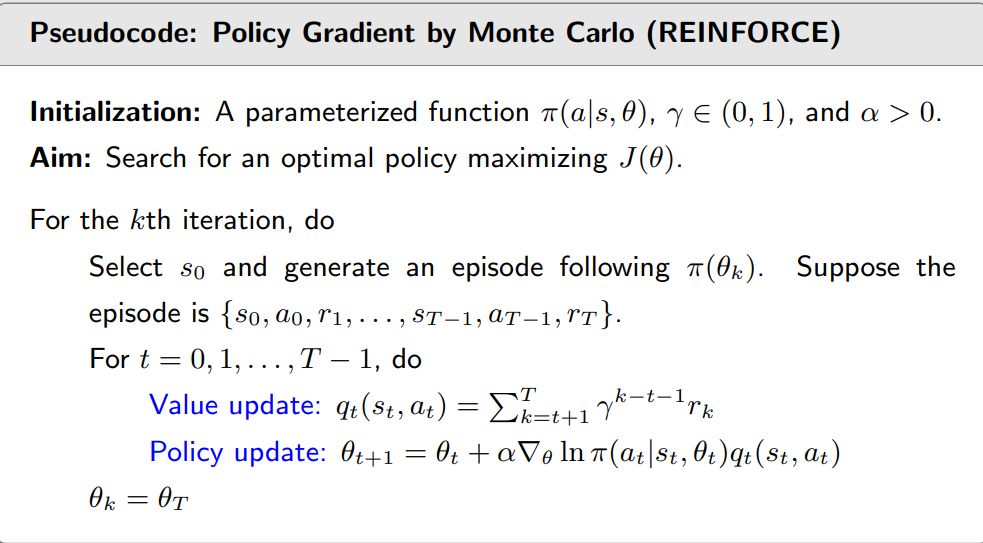
1：Monte-Carlo 对应Reinfoce

2：TD methods 对应 Actor-Critic

$$
\theta_{t+1}=\theta_{t}+\alpha \underbrace{\left(\frac{q_{t}\left(s_{t}, a_{t}\right)}{\pi\left(a_{t} \mid s_{t}, \theta_{t}\right)}\right)}{\beta{t}} \nabla_{\theta} \pi\left(a_{t} \mid s_{t}, \theta_{t}\right)
$$
The coefficient $\beta_{t}$ can well balance exploration and exploitation.

• First, $\beta_{t}$ is proportional to $q_{t}\left(s_{t}, a_{t}\right)$ .
• If $q_{t}\left(s_{t}, a_{t}\right)$ is great, then $\beta_{t}$ is great.（即return大的action，后续选到该action的概率就大！体现剥削性）
• Therefore, the algorithm intends to enhance actions with greater values.
• Second, $\beta_{t}$ is inversely proportional to $\pi\left(a_{t} \mid s_{t}, \theta_{t}\right)$ .
• If $\pi\left(a_{t} \mid s_{t}, \theta_{t}\right)$ is small, then $\beta_{t}$ is large.（即其他action 本身概率小的话，则后续选到他的概率会增大，体现探索性）
• Therefore, the algorithm intends to explore actions that have low probabilities.

伪代码！

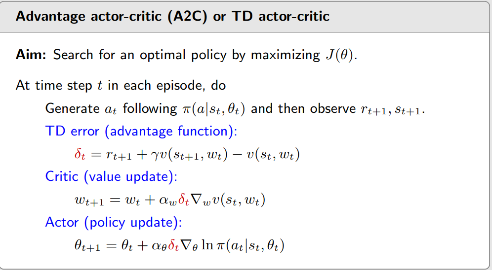
Actor-Critic Methods

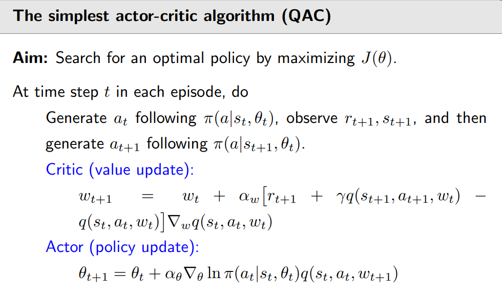
The Simplest AC（QAC）

实际是Policy gradient，只不过结合了value function

Core Idea：利用TD估计，称为actor-critic

何为actor：policy update

何为critic：policy evaluation

对应运用TD算法估计action-value的

A2C

Baseline invariance

Core Idea：introduce a baseline to reduce variance

$$
\begin{aligned}
\nabla_{\theta} J(\theta) & =\mathbb{E}{S \sim \eta, A \sim \pi}\left[\nabla{\theta} \ln \pi\left(A \mid S, \theta_{t}\right) q_{\pi}(S, A)\right] \ \
& =\mathbb{E}{S \sim \eta, A \sim \pi}\left[\nabla{\theta} \ln \pi\left(A \mid S, \theta_{t}\right)\left(q_{\pi}(S, A)-b(S)\right)\right]
\end{aligned}
$$
NOTE：该函数为S的函数，且添加后对期望没有影响，但会影响方差

relative proof
$$
\begin{aligned}
\mathbb{E}{S \sim \eta, A \sim \pi}\left[\nabla{\theta} \ln \pi\left(A \mid S, \theta_{t}\right) b(S)\right] & =\sum_{s \in \mathcal{S}} \eta(s) \sum_{a \in \mathcal{A}} \pi\left(a \mid s, \theta_{t}\right) \nabla_{\theta} \ln \pi\left(a \mid s, \theta_{t}\right) b(s) \
& =\sum_{s \in \mathcal{S}} \eta(s) \sum_{a \in \mathcal{A}} \nabla_{\theta} \pi\left(a \mid s, \theta_{t}\right) b(s) \
& =\sum_{s \in \mathcal{S}} \eta(s) b(s) \sum_{a \in \mathcal{A}} \nabla_{\theta} \pi\left(a \mid s, \theta_{t}\right) \
& =\sum_{s \in \mathcal{S}} \eta(s) b(s) \nabla_{\theta} \sum_{a \in \mathcal{A}} \pi\left(a \mid s, \theta_{t}\right) \
& =\sum_{s \in \mathcal{S}} \eta(s) b(s) \nabla_{\theta} 1=0
\end{aligned}
$$

• Why? Because $\operatorname{tr}[\operatorname{var}(X)]=\mathbb{E}\left[X^{T} X\right]-\bar{x}^{T} \bar{x}$ and

$$
\begin{aligned}
\mathbb{E}\left[X^{T} X\right] & =\mathbb{E}\left[\left(\nabla_{\theta} \ln \pi\right)^{T}\left(\nabla_{\theta} \ln \pi\right)\left(q_{\pi}(S, A)-b(S)\right)^{2}\right] \
& =\mathbb{E}\left[\left|\nabla_{\theta} \ln \pi\right|^{2}\left(q_{\pi}(S, A)-b(S)\right)^{2}\right]
\end{aligned}
$$

Imagine $b$ is huge (e.g., 1 millon)

b存在最优解，但由于过于复杂，我们一般用 $v_\pi(s)$替代

algorithm

$$
\begin{aligned}
\theta_{t+1} & =\theta_{t}+\alpha \mathbb{E}\left[\nabla_{\theta} \ln \pi\left(A \mid S, \theta_{t}\right)\left[q_{\pi}(S, A)-v_{\pi}(S)\right]\right] \
& \doteq \theta_{t}+\alpha \mathbb{E}\left[\nabla_{\theta} \ln \pi\left(A \mid S, \theta_{t}\right) \delta_{\pi}(S, A)\right]
\end{aligned}
$$

where

$$
\delta_{\pi}(S, A) \doteq q_{\pi}(S, A)-v_{\pi}(S)
$$
is called the advantage function (why called advantage?).

当 $q_\pi$大于 $v_{\pi}(S)$，说明该state action-pair优秀！

进行进一步变换
$$
\begin{aligned}
\theta_{t+1} & =\theta_{t}+\alpha \nabla_{\theta} \ln \pi\left(a_{t} \mid s_{t}, \theta_{t}\right) \delta_{t}\left(s_{t}, a_{t}\right) \
& =\theta_{t}+\alpha \frac{\nabla_{\theta} \pi\left(a_{t} \mid s_{t}, \theta_{t}\right)}{\pi\left(a_{t} \mid s_{t}, \theta_{t}\right)} \delta_{t}\left(s_{t}, a_{t}\right) \
& =\theta_{t}+\alpha \underbrace{\left(\frac{\delta_{t}\left(s_{t}, a_{t}\right)}{\pi\left(a_{t} \mid s_{t}, \theta_{t}\right)}\right)}{\text {step size }} \nabla{\theta} \pi\left(a_{t} \mid s_{t}, \theta_{t}\right)
\end{aligned}
$$
同样能平衡 exploration 和exploitation，而且更好，因为分子是相对值（作差），而QAC是绝对值

进一步，对应的$\delta_{\pi}(S, A)$可以由TD算法估计得到

伪代码：

由于已经是stochastic，所以不需要$ε$-greedy

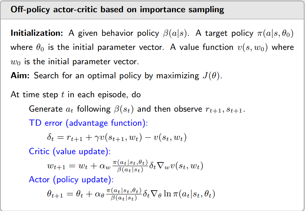
Off-policy AC

有两个概率分布，用其中一个概率分布计算另外一个概率分布的期望！

Example

$$
p_{0}(X=+1)=0.5, \quad p_{0}(X=-1)=0.5
$$

$$
p_{1}(X=+1)=0.8, \quad p_{1}(X=-1)=0.2
$$

The expectation is

$$
\mathbb{E}{X \sim p{1}}[X]=(+1) \cdot 0.8+(-1) \cdot 0.2=0.6
$$
If we use the average of the samples, then without suprising

$$
\bar{x}=\frac{1}{n} \sum_{i=1}^{n} x_{i} \rightarrow \mathbb{E}{X \sim p{1}}[X]=0.6 \neq \mathbb{E}{X \sim p{0}}[X]
$$

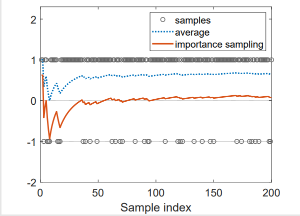
Importance sampling

Note that

$$
\mathbb{E}{X \sim p{0}}[X]=\sum_{x} p_{0}(x) x=\sum_{x} p_{1}(x) \underbrace{\frac{p_{0}(x)}{p_{1}(x)}}{f(x)} x=\mathbb{E}{X \sim p_{1}}[f(X)]
$$

• Thus, we can estimate $\mathbb{E}{X \sim p{1}}[f(X)]$ in order to estimate $\mathbb{E}{X \sim p{0}}[X]$ .
• How to estimate $\mathbb{E}{X \sim p{1}}[f(X)]$ ? Easy. Let（即对$f(x_i)$采样）

$$
\bar{f} \doteq \frac{1}{n} \sum_{i=1}^{n} f\left(x_{i}\right), \quad \text { where } x_{i} \sim p_{1}
$$

Then,

$$
\begin{array}{c}
\mathbb{E}{X \sim p{1}}[\bar{f}]=\mathbb{E}{X \sim p{1}}[f(X)] \
\operatorname{var}{X \sim p{1}}[\bar{f}]=\frac{1}{n} \operatorname{var}{X \sim p{1}}[f(X)]
\end{array}
$$
Therefore, $\bar{f}$ is a good approximation for $\mathbb{E}{X \sim p{1}}[f(X)]=\mathbb{E}{X \sim p{0}}[X]$

• $\frac{p_{0}\left(x_{i}\right)}{p_{1}\left(x_{i}\right)}$ is called the importance weight.
• If $p_{1}\left(x_{i}\right)=p_{0}\left(x_{i}\right)$ , the importance weight is one and $\bar{f}$ becomes $\bar{x}$ .
• If $p_{0}\left(x_{i}\right) \geq p_{1}\left(x_{i}\right), x_{i}$ can be more often sampled by $p_{0}$ than $p_{1}$ . The importance weight (>1) can emphasize the importance of this sample.
• 举个栗子：当$p_0 > p_1$时，说明原本这个样本概率较大，$p_0$较大，但是在 $p_1$内较少出现，因此很珍贵，要加大其比重！

off-policy gradient

• Suppose $\beta$ is the behavior policy that generates experience samples.
• Our aim is to use these samples to update a target policy $\pi$ that can minimize the metric

$$
J(\theta)=\sum_{s \in \mathcal{S}} d_{\beta}(s) v_{\pi}(s)=\mathbb{E}{S \sim d{\beta}}\left[v_{\pi}(S)\right]
$$

where $d_{\beta}$ is the stationary distribution under policy $\beta$ .

So ,in the discounted case where $\gamma \in(0,1)$ , the gradient of $J(\theta)$ is
$$
\nabla_{\theta} J(\theta)=\mathbb{E}{S \sim \rho, A \sim \beta}\left[\frac{\pi(A \mid S, \theta)}{\beta(A \mid S)} \nabla{\theta} \ln \pi(A \mid S, \theta) q_{\pi}(S, A)\right]
$$
where $\beta$ is the behavior policy and $\rho$ is a state distribution.

The algorithm

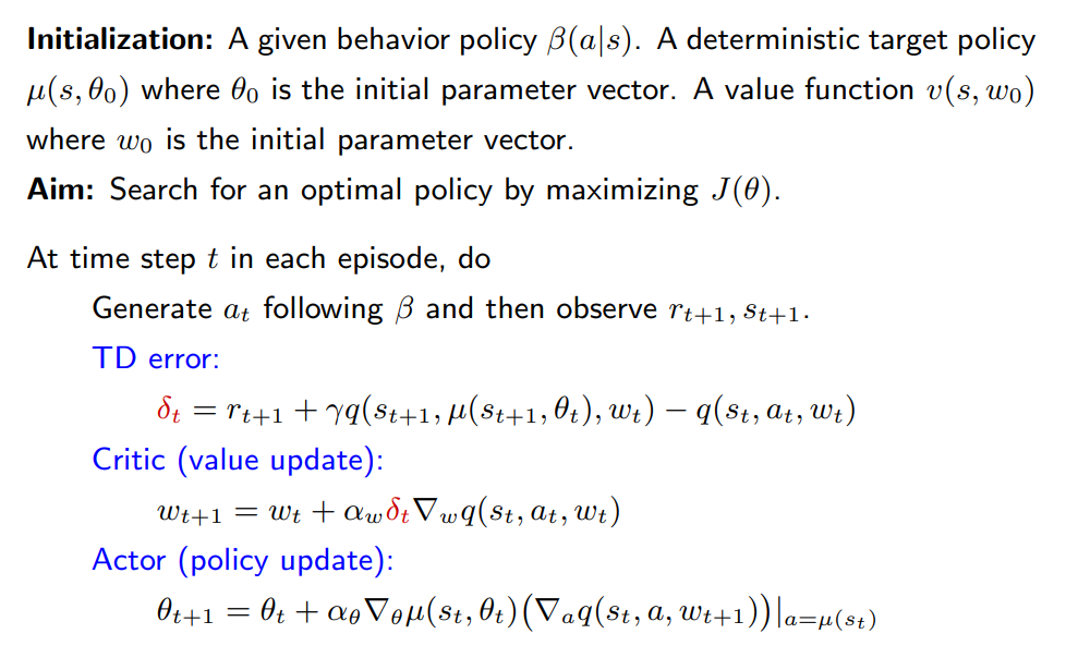
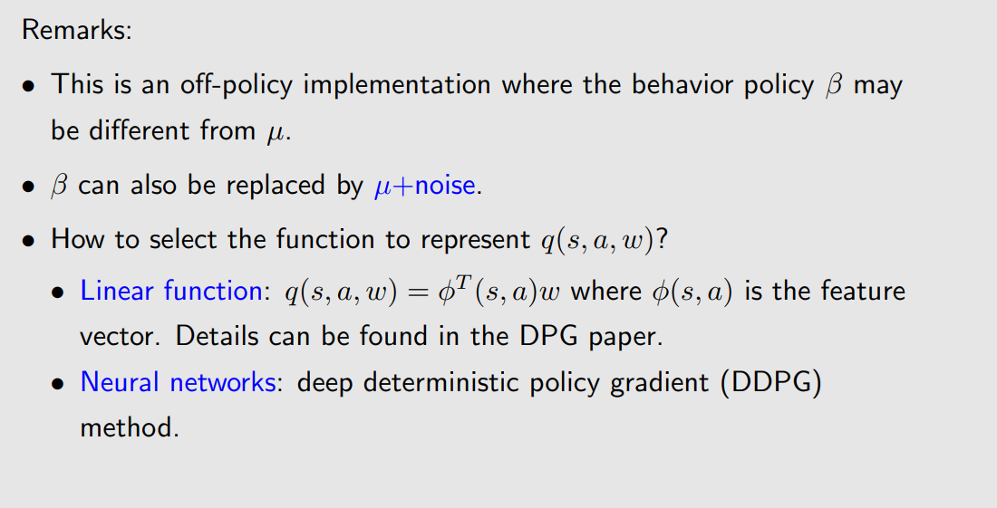
DPG

introduction

Up to now, the policies used in the policy gradient methods are all
stochastic since $π(a|s, θ)$ > 0 for every (s, a).
Can we use deterministic policies in the policy gradient methods?

• Benefit: it can handle continuous action.（即action有无数个，此时不能用随机的action，必须确定性的action）

• Now, the deterministic policy is specifically denoted as

$$
a=\mu(s, \theta) \doteq \mu(s)
$$

• $\mu$ is a mapping from $\mathcal{S}$ to $\mathcal{A}$ .（从state映射到action space，每个状态有确定性的动作）
• $\mu$ can be represented by, for example, a neural network with the input as $s$ , the output as $a$ , and the parameter as $\theta$ .
• We may write $\mu(s, \theta)$ in short as $\mu(s)$ .

deterministic policy gradient

$$
J(\theta)=\mathbb{E}\left[v_{\mu}(s)\right]=\sum_{s \in \mathcal{S}} d_{0}(s) v_{\mu}(s)
$$

where $d_{0}(s)$ is a probability distribution satisfying $\sum_{s \in \mathcal{S}} d_{0}(s)=1$ .

• $d_{0}$ is selected to be independent of $\mu$ . The gradient in this case is easier to calculate.
• There are two special yet important cases of selecting $d_{0}$ .
• • The first special case is that $d_{0}\left(s_{0}\right)=1$ and $d_{0}\left(s \neq s_{0}\right)=0$ , where $s_{0}$ is a specific starting state of interest.
• • The second special case is that $d_{0}$ is the stationary distribution of a behavior policy that is different from the $\mu$ .

In the discounted case where $\gamma \in(0,1)$ , the gradient of $J(\theta)$ is
$$
\begin{aligned}
\nabla_{\theta} J(\theta) & =\left.\sum_{s \in \mathcal{S}} \rho_{\mu}(s) \nabla_{\theta} \mu(s)\left(\nabla_{a} q_{\mu}(s, a)\right)\right|{a=\mu(s)} \
& =\mathbb{E}{S \sim \rho_{\mu}}\left[\left.\nabla_{\theta} \mu(S)\left(\nabla_{a} q_{\mu}(S, a)\right)\right|{a=\mu(S)}\right]
\end{aligned}
$$
Here, $\rho{\mu}$ is a state distribution.

algorithm

Over!